

Astrophotography filters: How narrow is too narrow
Saturday, June 29, 2024

|
Jim Thompson |
This investigative report about astrophotography filters delves into the optimal bandwidth for narrowband filters used in astrophotography of emission nebulae. Jim Thompson's comprehensive analysis explores improvements in contrast and signal-to-noise ratio (SNR), practical limitations, cost-effectiveness, and the impact of filter bandwidth on overall imaging performance.
For many years now I have been promoting the idea that for emission nebulae, whether you have light pollution (LP) or not, the narrower your filter’s pass bands are, the better. Time and again my test results have demonstrated this relationship to be true; that object contrast and signal-to-noise-ratio (SNR) increase as the pass band width decreases. Recently however a question occurred to me: is there no limit to this relationship, or is there a practical limit on how narrow a filter’s pass bands should be? The purpose of this test report is to document my investigation of the question “How narrow is too narrow?”
Objective of the report
The objective of this test report is to use several avenues of investigation to determine if there is an optimum filter bandwidth to use when imaging emission nebulae. The use of the term “bandwidth” in this report refers specifically to a filter's full-width half maximum (FWHM), the wavelength range over which the filter's transmissivity is more than 50% of its maximum. In my investigations, I have focused on H-α filters as a proxy for all narrowband filters and have considered FWHMs ranging from 100nm down to 0.1nm. Because H-α filters spanning this entire range are not readily available, I have used a combination of analysis and testing in my investigations.
Filter performance is evaluated in my analyses and testing based on the increase in contrast between the observed object and the background (see Equation 1) and SNR (Equation 2 & 3), both of which are measurable quantities. If the theory is born out in the analysis and test results, there should be an observable improvement in deep sky object contrast and SNR as I move to progressively narrower passbands. Whether there is a FWHM value that gives the maximum performance, or if performance continues to improve the narrower the FWHM, is to be determined. This is an important question as there is also an increase in filter cost as pass bands get narrower. Whether or not the increase in performance is worth the increase in cost is yet another question that will hopefully be answered during my investigations.
Equations:
Equation 1: %Contrast = (Lsky+object – Lsky) / Lsky * 100
, where: Lsky+object = Mean luminance of target object including LP contribution, and Lsky = Mean luminance of background sky with LP contribution.
Equation 2: SNR_theory = (Lsky+object – Lsky) / sqrt(Lsky+object + DC + RN2)
, where: DC = Dark current signal in units of luminance, and RN = RMS read noise in units of luminance.
Equation 3: SNR_measured = (Lsky+object – Lsky) / STDEVsky+object
, where STDEVsky+object = Standard deviation of target object luminance.
Method
Several different approaches were used in this investigation, as described below:
-
Use idealized numerical models of filters with FWHM from 100 to 0.1nm, and filter performance analysis method I developed in 2012, to predict filter performance for a range of conditions. This approach permitted consideration of filters that do not presently exist commercially and allowed a prediction of theoretically what is possible in terms of filter performance.
-
Use the same idealized numerical models to predict the impact of band shift on filter performance when used on a range of different telescope types and focal ratios. As filter pass bands become narrower, they become more susceptible to the band shift phenomenon. The degradation of filter performance with faster f-ratios is an important part of this investigation.
-
Survey available commercial filter spectrum data and evaluate their performance by analysis against the idealized models. The current availability of narrowband filters and their relative performance compared to what is theoretically possible provides some indication of the feasibility of producing very narrow filters commercially.
-
Image test a subset of the commercially available filters to determine how their measured performance compares to predictions.
-
Survey pricing data for commercially available filters and combine them with performance data to establish a price-performance index. Include comprehensive market data for all available brands of filters, not just those for which detailed spectrum data is available.
The numerical method used for predicting filter performance uses the detailed measured filter spectra combined with the emission spectrum of typical LP, the spectral response of an assumed camera sensor, and the emission spectrum of a typical H-α rich emission nebula to predict the integrated luminance of the sky and sky-plus-object as perceived by the camera. Most of the detailed filter transmission spectrum data used was measured in my basement workshop with an Ocean Insight USB4000 spectrometer and a broad-spectrum light source. Filter spectra were measured for a range of filter angles relative to the light path, from 0° (perpendicular) to 20° off-axis. The spectrometer was recently upgraded, replacing the entrance slit and diffraction grating, to give a wavelength resolution of 0.5nm. Image testing was performed from my backyard in central Ottawa, Canada (Bortle 9+, NELM +2.9). Camera and telescope combinations varied depending on the test day and test object:
Astrophotography filters imaging sessions
- Session 1: June 12th, 2022; IC1318 “Asian Dragon Nebula”; Mallincam DS432M-TEC (bin 1x1) monochrome camera; William Optics FLT98 triplet apochromatic refractor (f/6.3).
- Session 2: June 16th, 2022; IC1318 “Asian Dragon Nebula”; ZWO ASI183MM Pro (bin 2x2) monochrome camera; William Optics FLT98 triplet apochromatic refractor (f/6.3).
- Session 3: June 24th, 2022; IC1318 “Asian Dragon Nebula”; ZWO ASI183MM Pro (bin 2x2) monochrome camera; William Optics FLT98 triplet apochromatic refractor (f/6.3).
- Session 4: June 28th, 2022; IC1318 “Asian Dragon Nebula”; Mallincam DS432M-TEC (bin 1x1) monochrome camera; Askar FMA230 triplet apochromatic refractor (f/4.6).
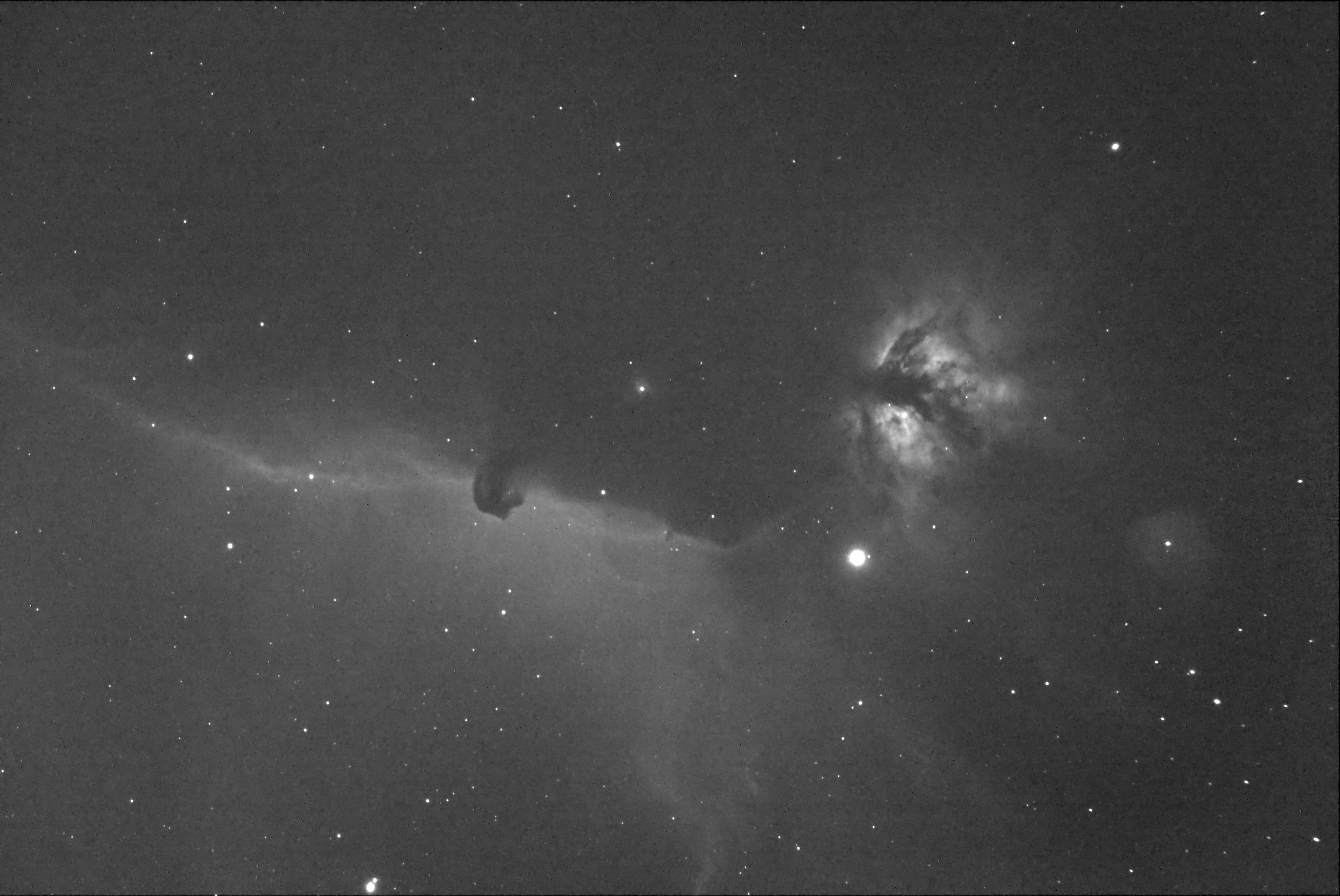
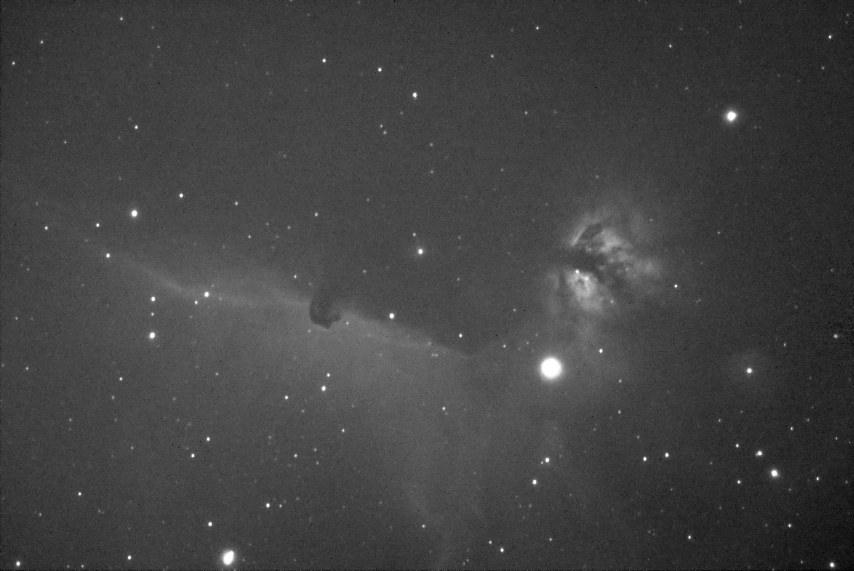
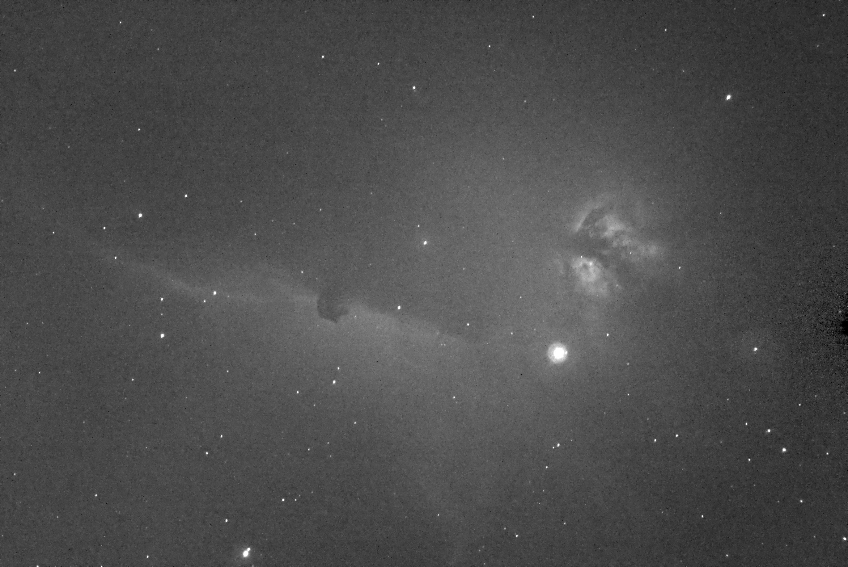
- Session 5: February 6th, 2023; B33 “Horsehead Nebula”; ZWO ASI183MM Pro (bin 2x2) monochrome camera; William Optics ZS66 ED doublet refractor (f/5.9).
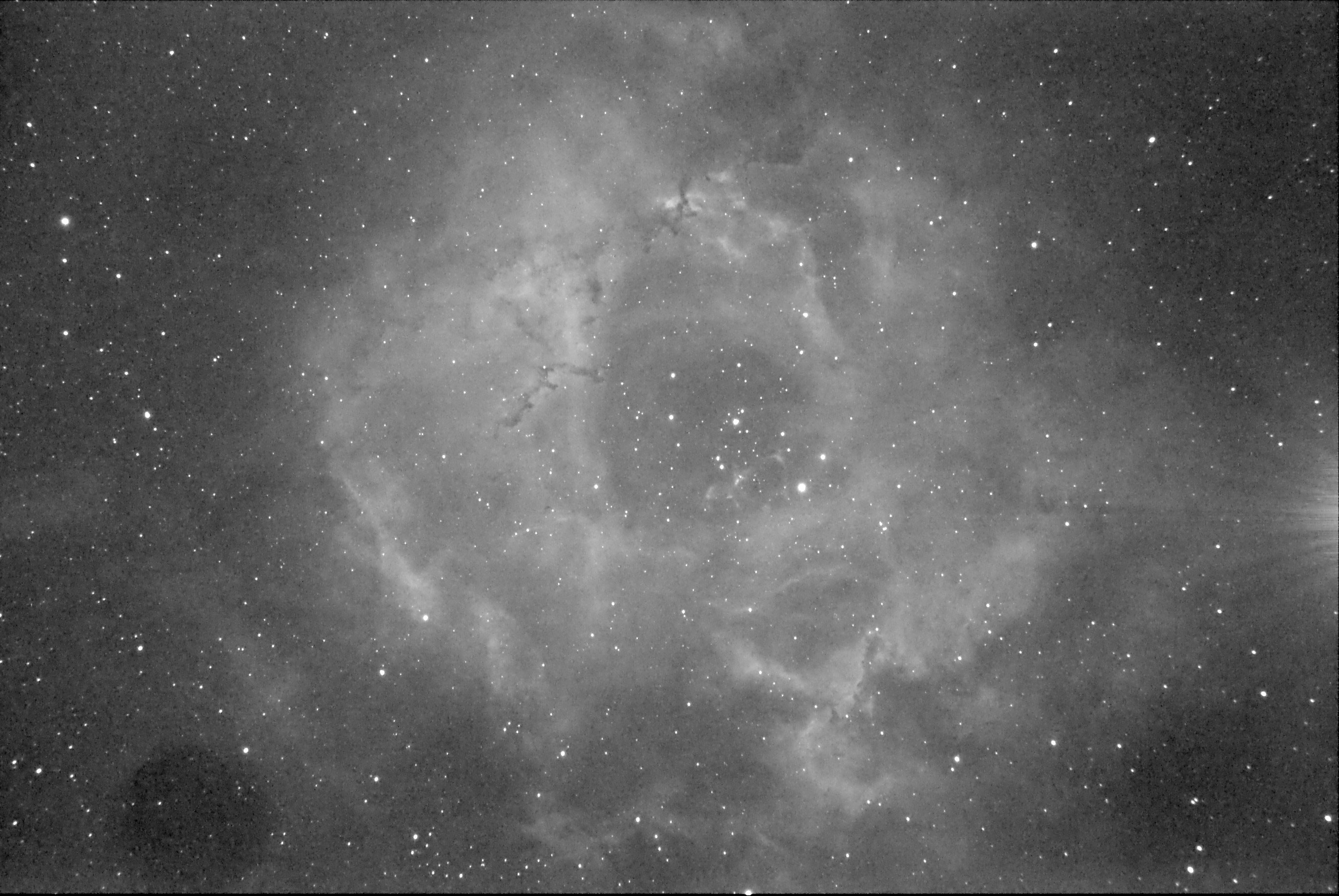
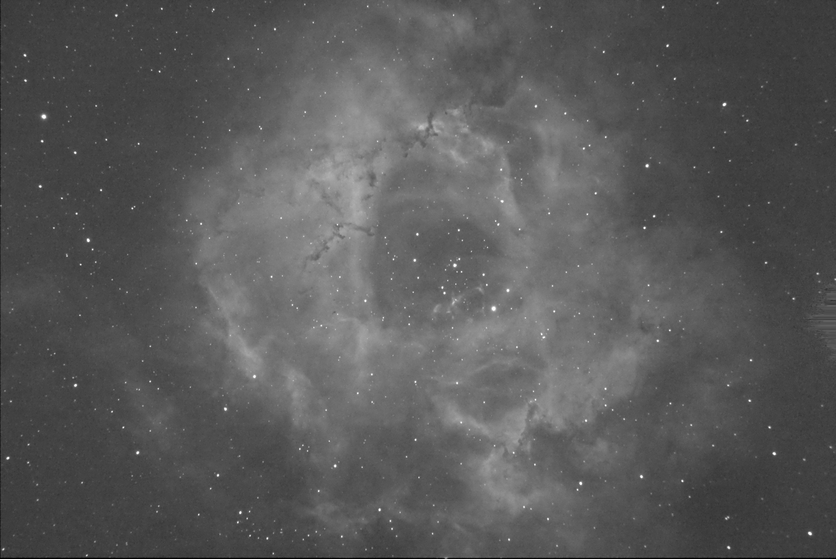
- Session 6: February 8th, 2023; NGC2244 “Rosette Nebula”; ZWO ASI183MM Pro (bin 2x2) monochrome camera; William Optics ZS66 ED doublet refractor (f/5.9).
- Session 7: July 27th, 2023; IC1318 “Asian Dragon Nebula”; Mallincam DS432M-TEC (bin 1x1) monochrome camera; William Optics FLT98 triplet apochromatic refractor (f/6.3).
- Session 8: August 1st, 2023; IC1318 “Asian Dragon Nebula”; Mallincam DS432M-TEC (bin 1x1) monochrome camera; Askar FMA230 triplet apochromatic refractor (f/4.6).
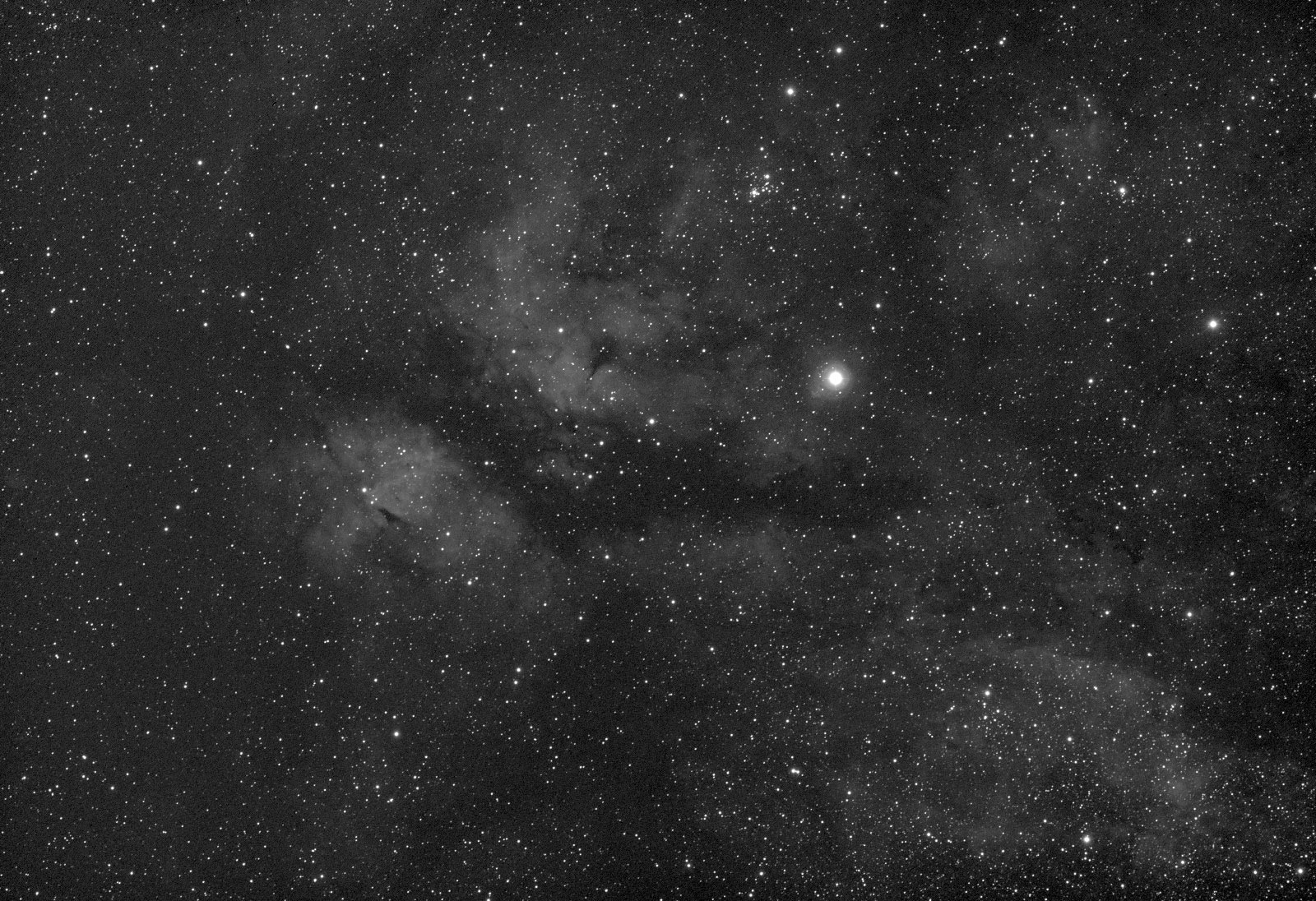
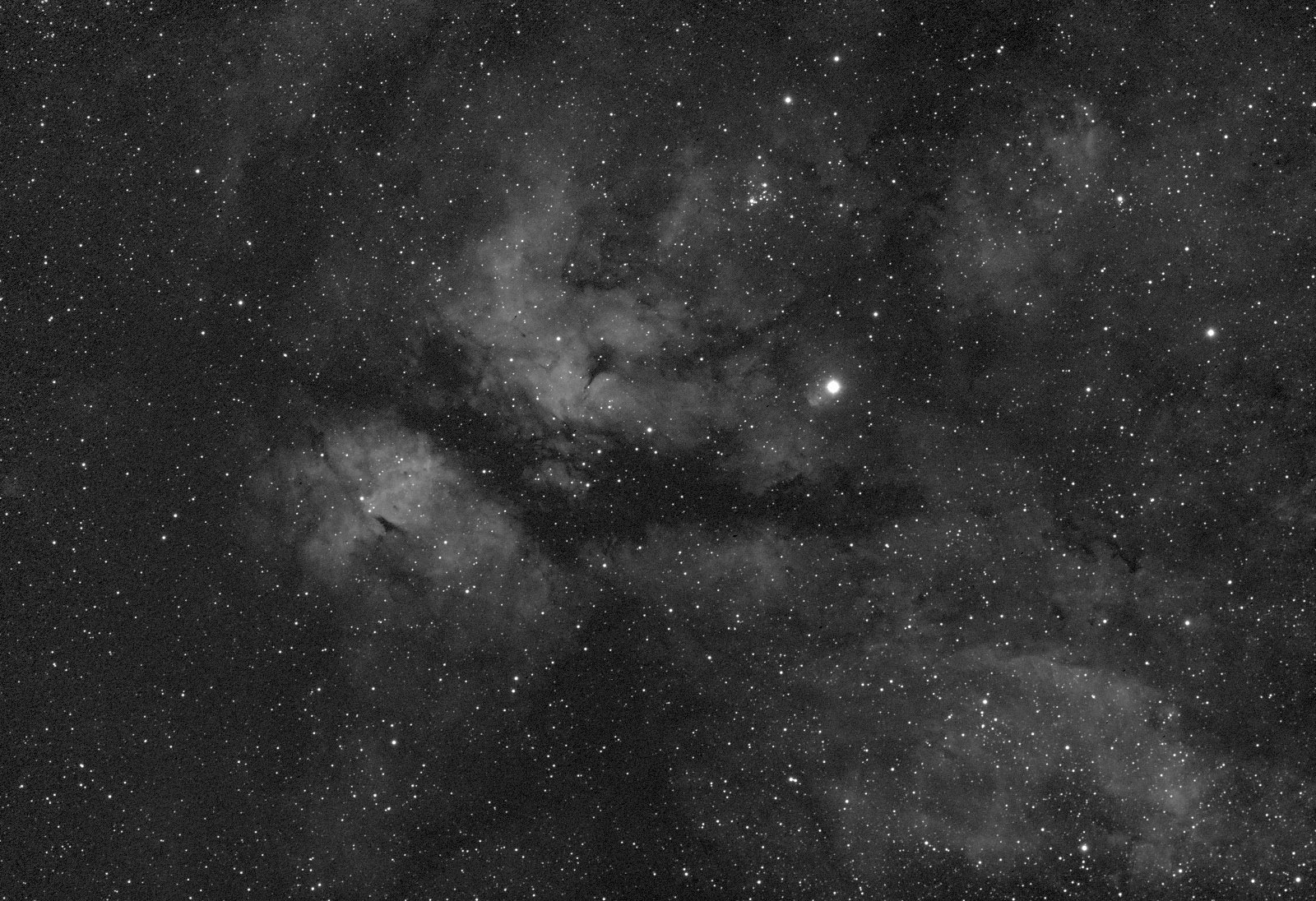
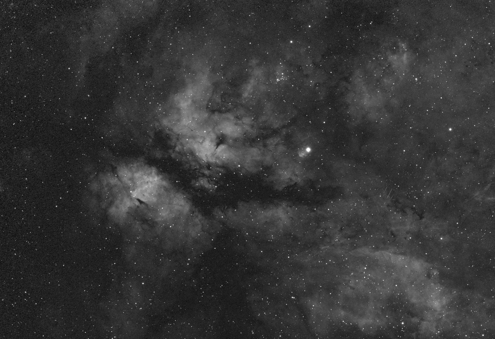
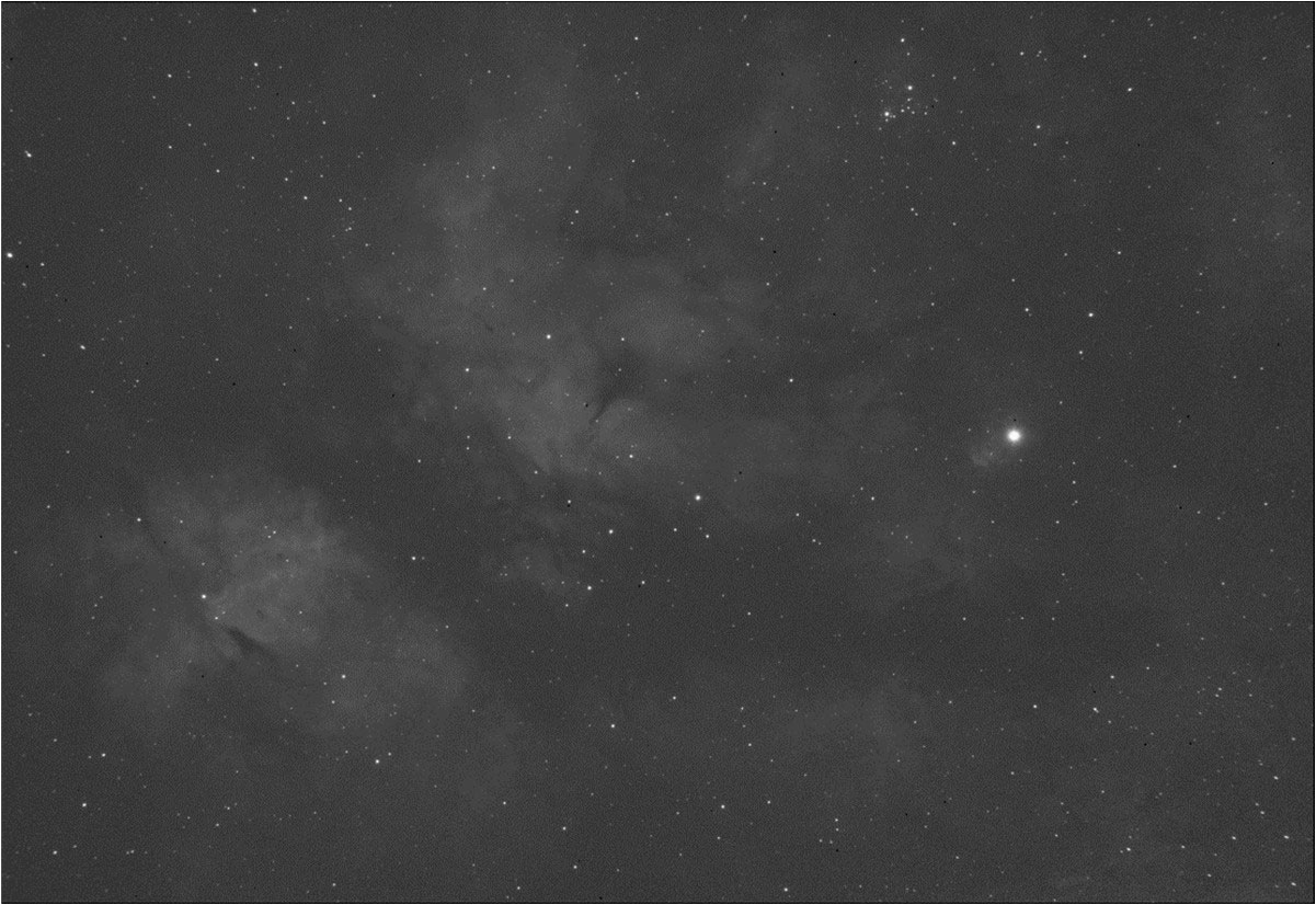
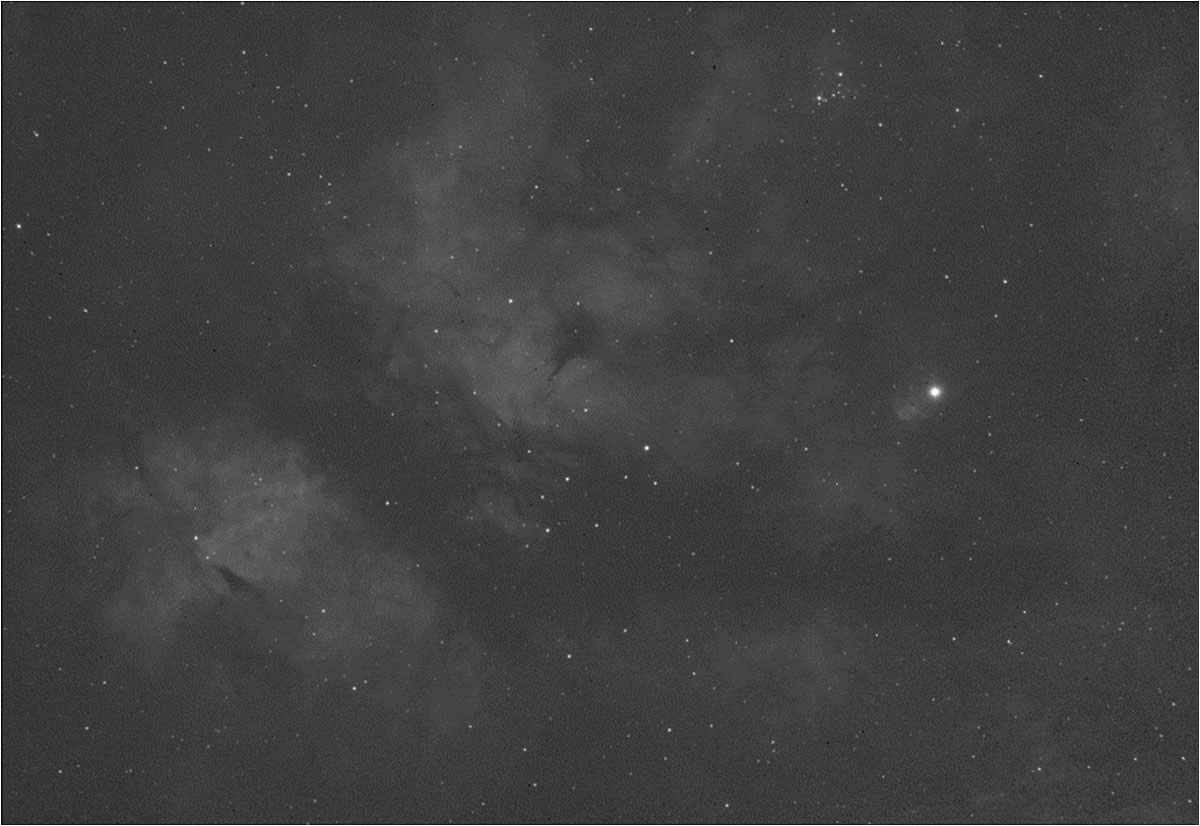
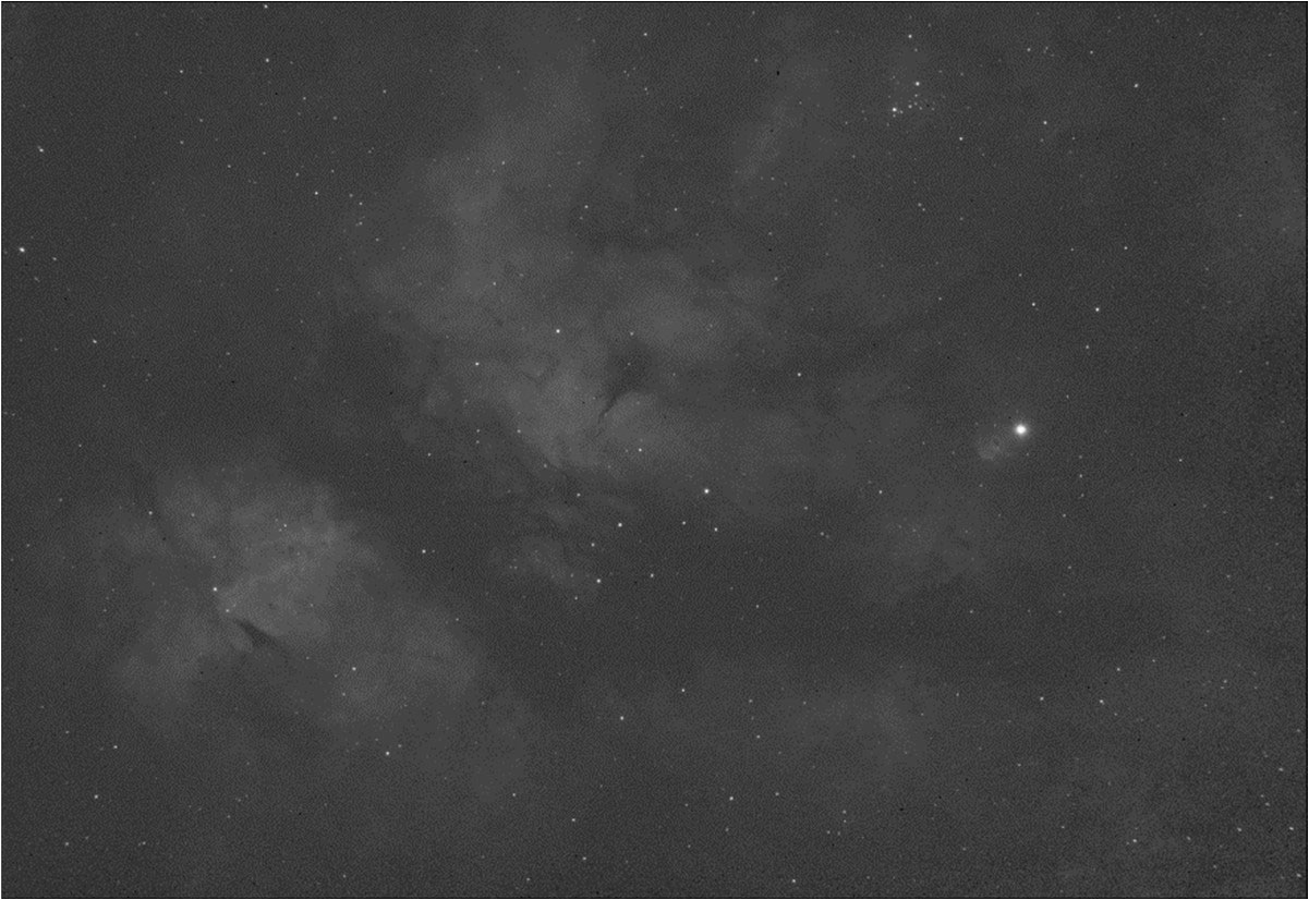
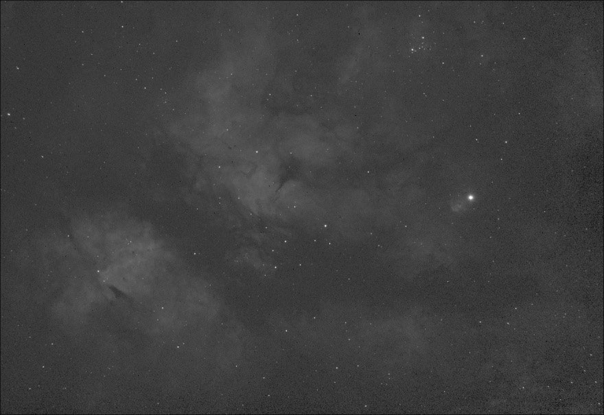
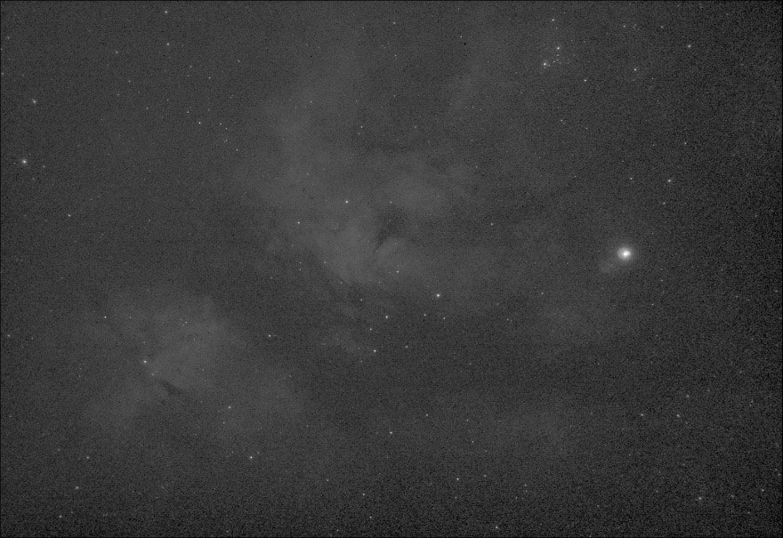
Note, IC1318 is more commonly known as the Butterfly or γ-Cygni nebula, but I think it looks like an Asian dragon and refers to it as such. This object is well suited for testing as it is placed directly overhead during summertime from my location.
Nebula reference spectrum
The filter performance prediction method that I use relies on a reference emission spectrum for the deep sky object the filter is being evaluated against. Sources for such reference spectra are readily available online. In particular, I have up until recently used spectra for NGC7000 (North American) and M27 (Dumbbell) as the references in my calculations. Something that I overlooked in the first version of this report is how the resolution of the spectrometer used to capture the reference spectra impacts the outcome of my analysis. For the filter performance predictions I have performed previously the impact of a low spectrum resolution has been negligible, but for this test report, the impact is significant due to the unusually narrow filter pass bands being considered. The impact of spectrum resolution is illustrated in Figure 1. The plot has the portion of an emission nebula’s spectrum from two different sources plotted around the H-α emission band. The red curve is representative of the reference spectrum data I had been using up until recently. It was captured by the well-known amateur astronomer Christian Buil using a spectrometer with a reported spectral resolving power of R=800. That translates to a wavelength resolution of 0.8nm in the H-α part of the spectrum. As a result of this instrument’s wavelength resolution, the emission lines of the nebula are artificially broadened. The blue curve is taken from a scientific paper where the authors used data gathered by the VLT UVES echelle spectrograph at the European Southern Observatory (ESO) in Chile. That instrument has a spectral resolving power of R=8800, giving a wavelength resolution of 0.07nm. That instrument is able to resolve the actual width of the nebula emission lines, and in fact uses this information to determine things like how fast the gas is moving or its temperature. The impact of the emission nebula spectrum resolution on my calculations is made evident by overlaying the transmissivity spectra for three of the idealized filters I have considered in my study. If the low-resolution nebula spectrum were to be used, filters with FWHM less than 2nm would not able to pass all of the H-α emission unhindered. This explains why in the first version of this report I was predicting that the theoretical maximum SNR is achieved for bandwidths around 1 to 2nm. If the high-resolution nebula spectrum is used for my predictions, the filter bandwidth would need to be below 0.2nm before the filter performance is noticeably impacted by all of the nebula emission not being passed.
Figure 1 Measured Nebula Emission Spectra @ Different Spectral Resolving Powers
Ideal filter predictions
To investigate whether or not there is an optimum filter bandwidth by the test would require possession of a very large number of filters, filters with FWHM values much smaller than are readily available from commercial retailers. Having custom filters made for the purpose of testing is possible but would be prohibitively expensive. Thus, I decided to investigate the problem using a numerical approach. A series of idealized H-α filter spectra were created, spanning the FWHM range of 0.1nm to 100nm. Figures 2 and 3 illustrate the appearance of the idealized filter spectra. These filter spectra were then run through my filter performance calculations to predict how they would perform in terms of contrast increase and SNR relative to no filter for three different LP levels.
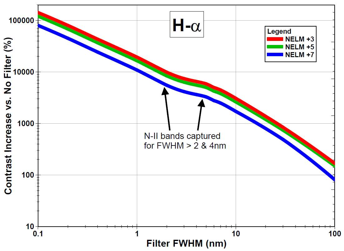
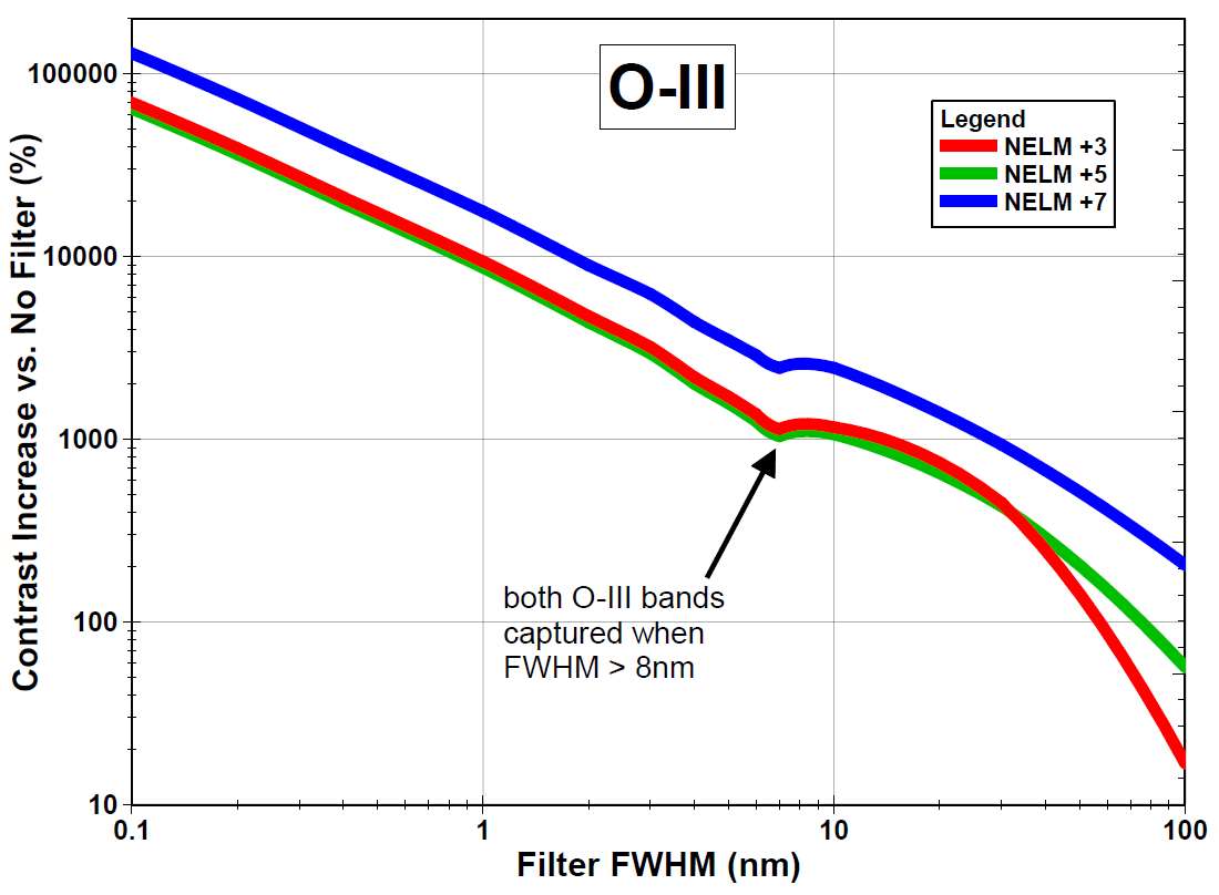
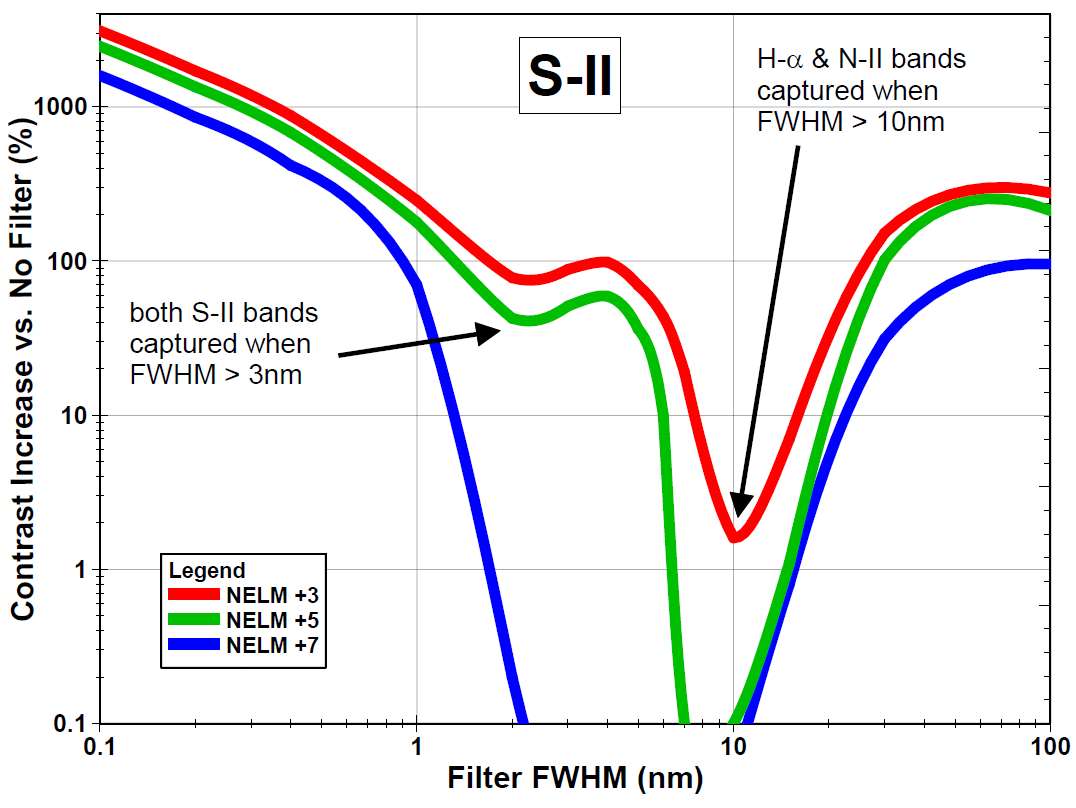
The first parameter to look at is the predicted contrast increase, which is presented in Figure 4. The predictions suggest that there is a relatively constant increase in contrast as FWHM decreases. There is a small joggle in performance predicted in the 2 to 4nm range that is a result of the filter passing or not passing the two N-II emission bands that are adjacent to the H-α emission band. Otherwise, there appears to be no maximum; contrast increases monotonically with decreasing bandwidth. Out of curiosity I also generated the same plot for O-III and S-II filters. They can be found in Appendix A at the end of this report.
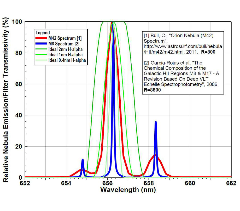
Figure 2 Idealized H-α Filter Spectra - A Figure 3
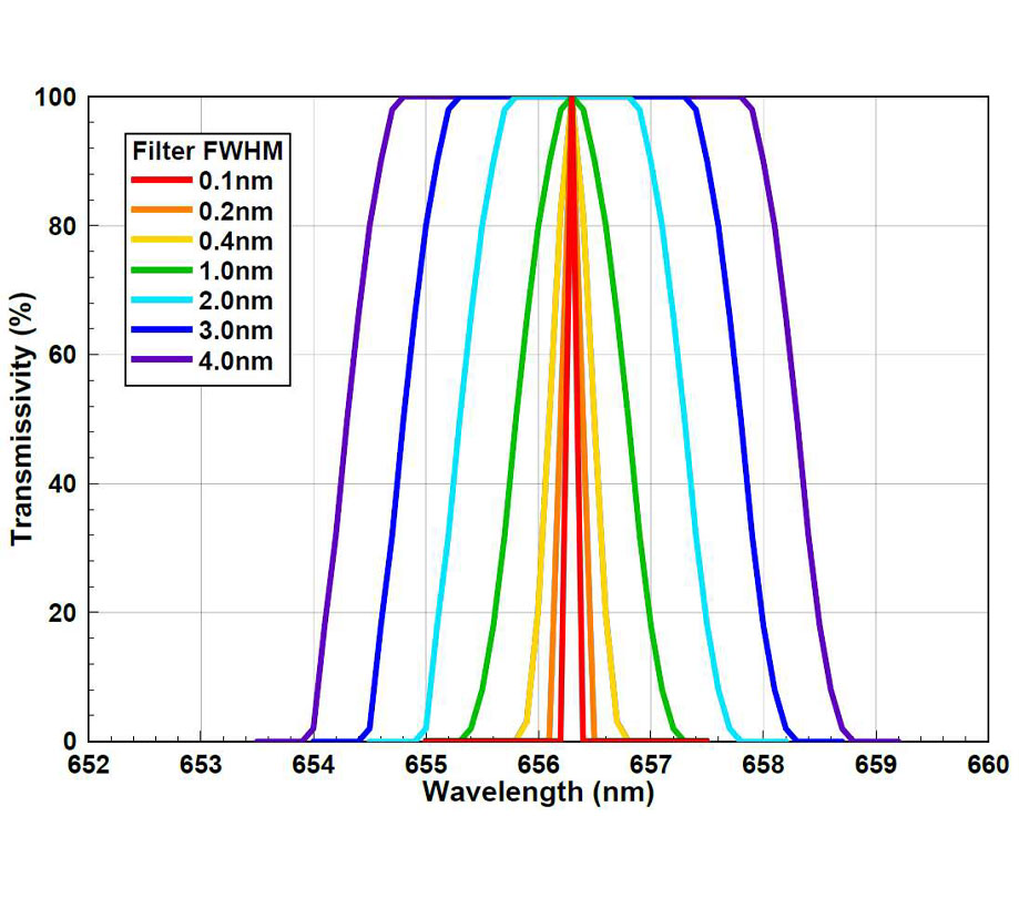
Figure 3 Idealized H-α Filter Spectra - B
Figure 4 Predicted Contrast Increase vs. Filter FWHM – Idealized Filters
The second parameter to look at is the predicted SNR, which is presented in Figure 5. SNR has been normalized against the no-filter case so that a value greater than 1.0 means the filter improves SNR. The predictions are plotted not only for three different LP levels but also for four different noise levels. Referring back to Equation 2, the noise is calculated using the square root of the sky+object signal plus additional noise from the dark current signal (DC) and RMS read noise (R). I have arbitrarily varied the DC+R contribution, expressing it as a fraction of the sky+object signal noise component. When the DC+R contribution to noise is zero, the SNR curve has a similar shape to the contrast curve, increasing in magnitude with decreasing bandwidth with a joggle around 2 to 4nm resulting from the two N-II emission bands. As the contribution of DC+R increases the curves flatten out; the advantage of a narrower bandwidth diminishes as the magnitude of the noise gets closer to the magnitude of the object signal. Similarly, the curves flatten as the LP level reduces. Due to the influence of the N-II emission bands, there would seem to be a sweet spot between 3 and 5nm where the SNR is about the same and at a maximum. A higher SNR could be achieved with a filter narrower than 2nm, but the result will be highly dependent on the LP level, dark current, and read noise. I also generated the same plot for O-III and S-II filters. They can be found in Appendix A at the end of this report.
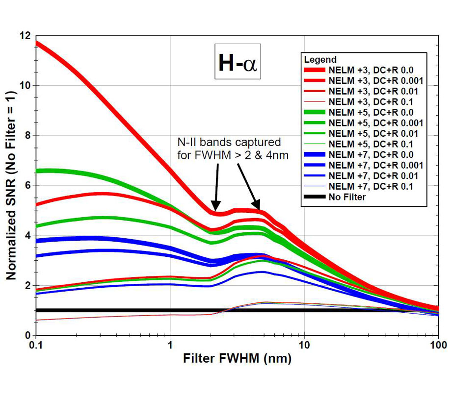
Figure 5 Predicted SNR vs. Filter FWHM – Idealized Filters
Ideal filter f-ratio sensitivity
Narrowband filters are made up of many alternating layers of refractory material and function as a result of the wave behavior of light, with constructive interference allowing the desired wavelengths through and destructive interference blocking the undesired wavelengths. As your scope optics get faster, the angle of light passing through the filter increases resulting in the effective thickness of the filter layers increasing and causing the filter transmission curves like those shown in Figures 2 and 3 to shift down and left. As a result, net filter transmission for the wavelength of interest goes down with decreasing f-ratio. Another way to look at the impact of using a narrowband filter on fast optics is it is like adding an aperture mask to your telescope. The narrower the filter, or the faster the optics, the smaller the effective aperture mask. This relationship is illustrated in Figures 6 to 8 for a range of generic filter bandwidths and optics f-ratios. Scopes with a central obstruction are especially affected since they have a larger percentage of their light cone at an angle away from the perpendicular. Note that the plots in Figures 6 to 8 are from one of my previously released technical reports: “Narrowband Filters & Fast Optics”, November 2020. I believe there are few people out there who would be willing to accept the severe reduction in effective aperture that accompanies filters with bandwidths less than 1nm. The increase in exposure time necessary to achieve the same SNR result as a wider filter makes them not worth any benefit to contrast that may be realized. There is a lot of room for optimizing the filter to one’s optics in the 1 to 10nm bandwidth range, and pre-shifted filters exist on the market to make sub-5nm filters attractive to fast scope users.
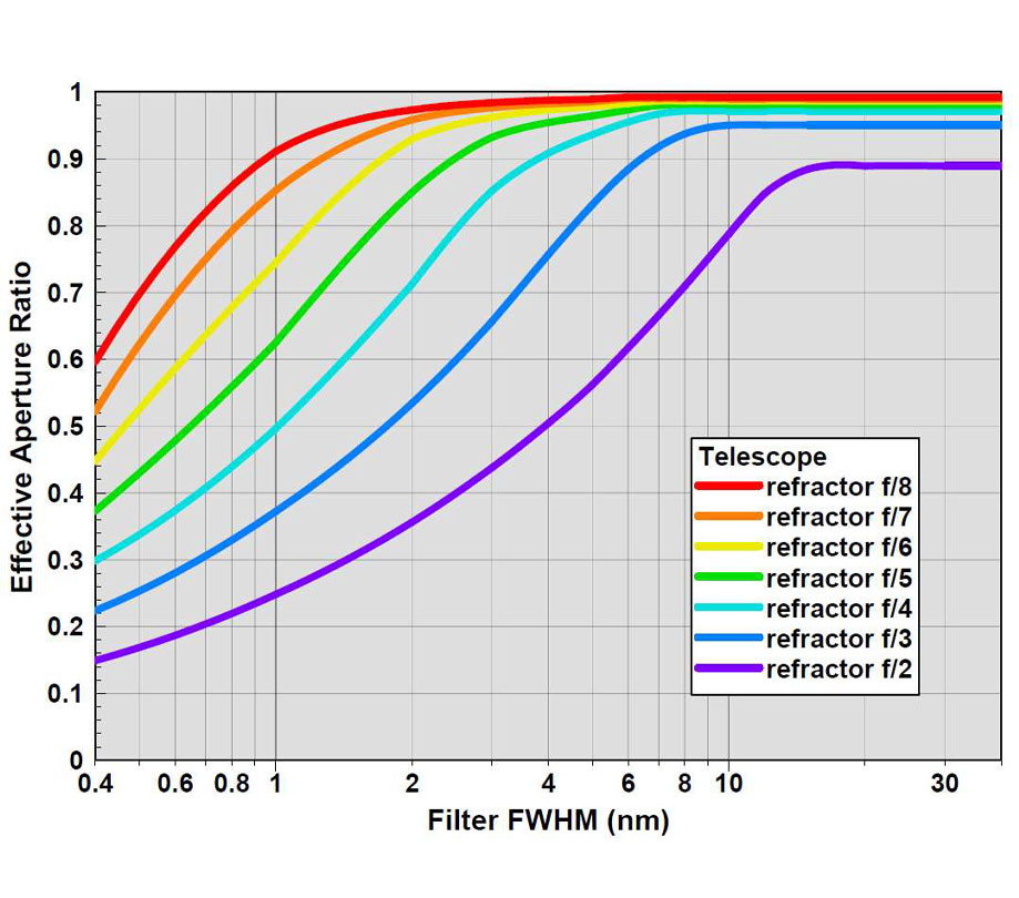
Figure 6 Predicted Effect of Filter Band Shift in Terms of Effective Aperture - Refractors
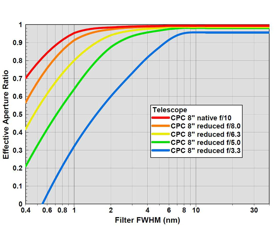
Figure 7 Predicted Effect of Filter Band Shift in Terms of Effective Aperture - SCTs
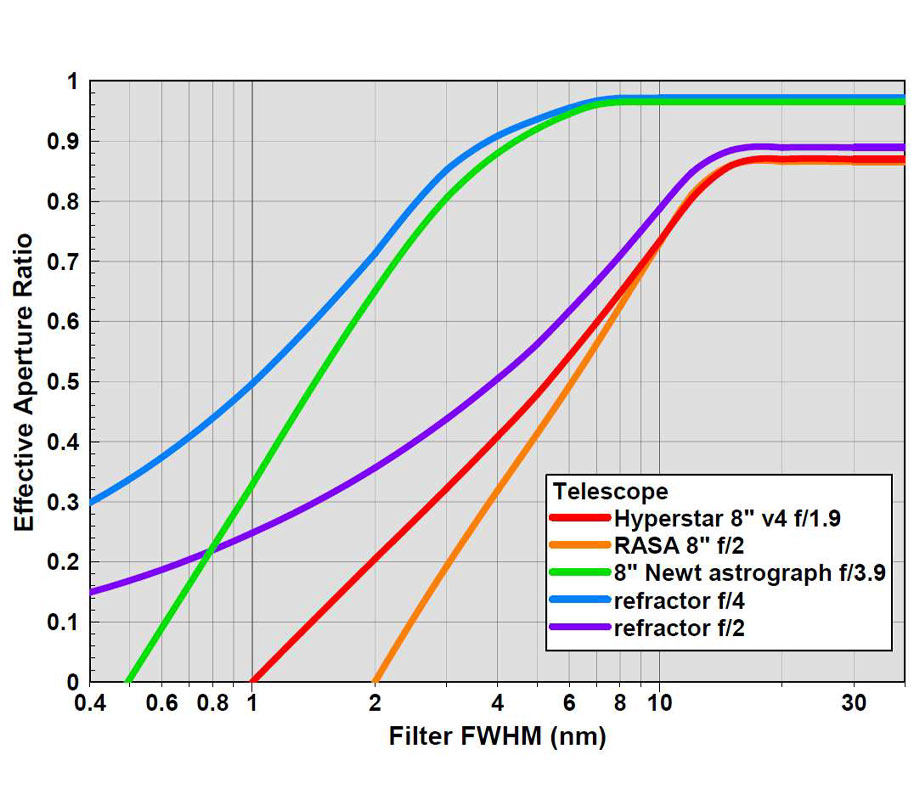
Figure 8 Predicted Effect of Filter Band Shift in Terms of Effective Aperture – Astrographs
Available filter performance predictions
I had a long list of H-α filters to choose from for this project, either in physical form or just as a measured spectrum data set. The list of filter configurations considered in this performance comparison is summarized in Table 1 (costs are for 2” version). Indicated in the table is the source used for each filter’s spectrum data, either a measurement made by myself (JT), the well-known amateur astronomer André Knöfel (AK), or by the manufacturer in the case of some Chroma brand filters (C). The values of FWHM quoted in the table are as I have calculated from each filter’s measured spectrum data. Also indicated in the table is whether or not I own a sample of the filter, and if I used it to collect image data as part of this test. Take note of the filter numbering in Table 1 as it will be used throughout the report.
Table 1 - List of filters considered in test
| No. | Filter or Filter Combo | FWHM [nm] | Cost [USD] | Have Sample [Y/N] | Spectra By [JT/AK] | Image Data [Y/N] |
|---|---|---|---|---|---|---|
| 0 | No Filter (for reference) | n.a. | 0 | Y | n.a. | Y |
| 1 | Optolong Nightsky H-α | 140 | 119 | Y | JT | Y |
| 2 | Optolong NS H-α + Astronomik UV/IR Cut | 67.0 | 218 | Y | JT | Y |
| 3 | Omega XMV660/40 | 43.6 | 180 | Y | JT | Y |
| 4 | IDAS NB-1 + Optolong NS H-α | 22.0 | 318 | Y | JT | Y |
| 5 | Omega 650BP10 | 11.3 | 220 | Y | JT | Y |
| 6 | Omega 8nm H-α | 7.7 | 180 | Y | JT | Y |
| 7 | Optolong 7nm H-α | 6.4 | 259 | Y | JT | Y |
| 8 | IDAS 6.8nm H-α | 6.7 | 379 | Y | JT | Y |
| 9 | IDAS 6.8nm H-α + Omega 650BP10 | 5.0 | 599 | Y | JT | Y |
| 10 | Antlia EDGE Narrowband H-α | 4.2 | 290 | Y | JT | Y |
| 11 | Optolong 3nm H-α | 3.1 | 439 | Y | JT | Y |
| 12 | Chroma 3nm H-α | 2.7 | 1300 | Y | JT | Y |
| 13 | Antlia Ultra Narrowband H-α | 2.1 | 590 | Y | JT | Y |
| 14 | Omega 1.5nm H-α (1") | 1.5 | 480 | Y | JT | Y |
| 15 | Andover 1nm H-α (1") | 1.2 | 563 | Y | JT | Y |
| 16 | Baader Planetarium 35nm H-α | 35.9 | 220 | N | AK | N |
| 17 | Astronomik 13nm H-α | 19.1 | 287 | N | AK | N |
| 18 | Chroma 8nm H-α | 7.7 | 830 | N | C | N |
| 19 | Baader Planetarium 7nm H-α | 6.9 | 279 | N | AK | N |
| 20 | Astronomik 6nm H-α | 6.3 | 470 | N | AK | N |
| 21 | Chroma 5nm H-α | 5.1 | 975 | N | C | N |
| 22 | Custom Scientific 4nm H-α | 5.0 | 1200 | N | AK | N |
Using my spectrometer, the spectral transmissivity for each filter that I have a sample of was measured for a range of filter angles relative to the light path. Figures 9 to 12 present plots of the resulting spectral transmissivity data for the case of the filter perpendicular to the light path. All the filters have their pass bands well positioned around 656nm, apart from a few exceptions. It is evident from the measured spectra that both the Baader 35nm H-α and Omega 650BP10 filters are not optimized for H-α as their center wavelength (CWL) is shifted significantly to the left, a property that would make them both sensitive to band shift. Similarly, my sample of the Optolong 7nm and Omega 1.5nm filters are also not properly centered on 656nm, being shifted significantly off-band to the right, which would actually mean these two filters should perform better at faster f-ratios.
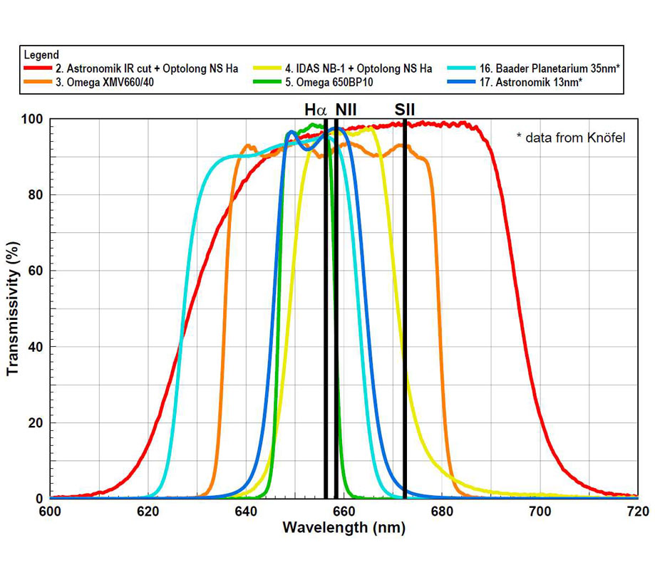
Figure 9 Measured Filter Spectra – Filter Perpendicular to Light Path, FWHM >10nm
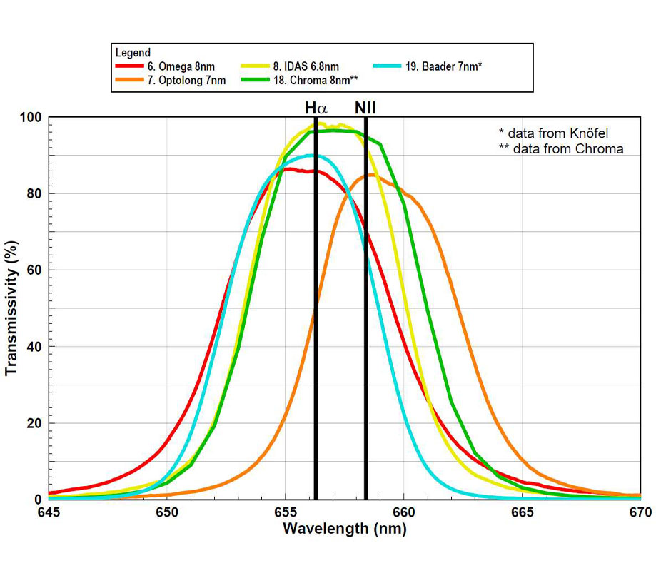
Figure 10 Measured Filter Spectra – Filter Perpendicular to Light Path, FWHM 6-10nm
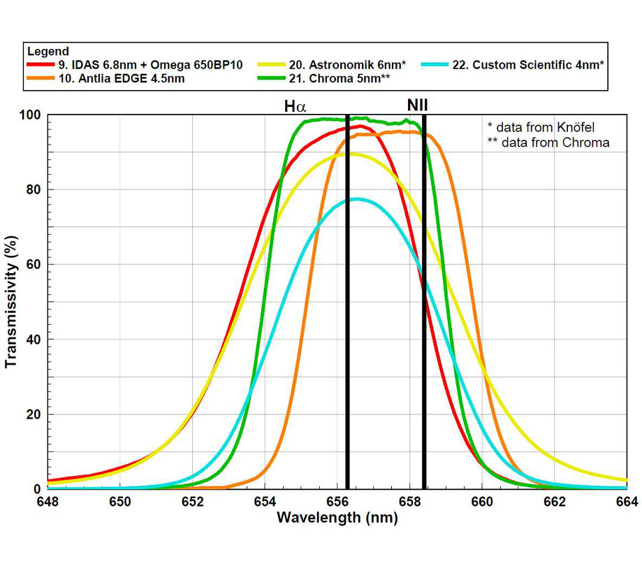
Figure 11 Measured Filter Spectra – Filter Perpendicular to Light Path, FWHM 3-6nm
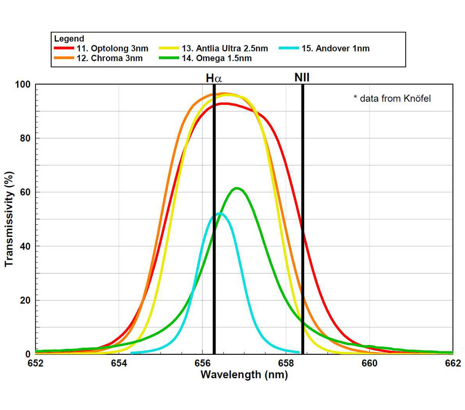
Figure 12 Measured Filter Spectra – Filter Perpendicular to Light Path, FWHM <3nm
The impact of the angle on transmission for each of the filters for which I have a sample is shown in Figures 13 and 14. As expected, filters with wide pass bands were less sensitive to angle than filters with narrow passbands, with the most sensitive filters to angle being the two sub-2nm samples. The Omega 650BP10 has almost the same sensitivity to angle as the 3nm filters because of its CWL being shifted to the left of 656nm. Similarly, the Optolong 7nm filter has performance that peaks at faster f-ratios because its CWL is shifted to the right. Figures 13 and 14 also have black vertical lines corresponding to different optics f-ratios. These lines are positioned at the angle values corresponding to light coming from the outer edge of the scope’s aperture for the noted f-ratio. The net performance of a filter on any particular speed of optics is an area weighted average of the filter’s performance, for light angles from perpendicular out to the angle at the outer edge of the aperture.
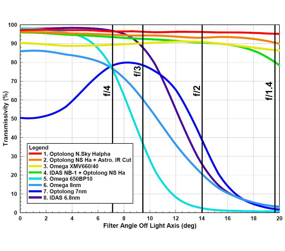
Figure 13 Measured Impact of Angle on Filter Response, FWHM >6nm
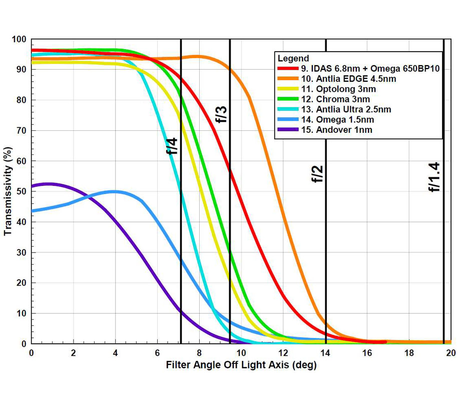
Figure 14 Measured Impact of Angle on Filter Response, FWHM <6nm
With the filter spectra in hand, it was possible to extract overall performance-related statistics for each filter, such as transmission values at key wavelengths of interest and pass bandwidths. These filter statistics are provided in Table 2, including a calculated value for percent Luminous Transmissivity (%LT), a single number that describes generally how much light is getting through the filter. The calculated value of %LT depends on the spectral response of the detector, which in this case is assumed to be a modern back-illuminated monochrome CMOS sensor. For the filters that I measured myself, I have included transmission measurements in the table for a range of telescope f-ratios, from f/∞ (perfectly parallel & perpendicular light) down to f/2.
Table 2 - Measured filter performance summary
| No. | Filter | Scope Optics | %LT* | Halpha Pass Band FWHM | Halpha (656.3) | N-II (658.4) | S-II (672.4) |
|---|---|---|---|---|---|---|---|
| 1 | Optolong Night Sky H-α | f/∞ | 37.9% | ~140nm (high pass filter) | 97.1% | 97.8% | 99.5% |
| f/6.3 | 97.2% | 97.4% | 99.3% | ||||
| f/4.9 | 97.1% | 97.4% | 99.2% | ||||
| f/3.0 | 96.7% | 97.0% | 98.8% | ||||
| f/2 | 96.3% | 96.7% | 98.6% | ||||
| 2 | Optolong NS H-α + Astronomik UV/IR | f/∞ | 13.1% | 67.0nm | 96.2% | 96.9% | 98.5% |
| Blocker | f/6.3 | 95.6% | 96.0% | 97.9% | |||
| f/4.9 | 95.4% | 95.6% | 97.8% | ||||
| f/3.0 | 94.9% | 95.1% | 97.2% | ||||
| f/2 | 94.1% | 94.3% | 96.3% | ||||
| 3 | Omega XMV660/40 | f/∞ | 8.29% | 43.6nm | 90.3% | 92.1% | 92.5% |
| f/6.3 | 89.1% | 90.7% | 91.1% | ||||
| f/4.9 | 89.0% | 90.7% | 90.7% | ||||
| f/3.0 | 89.4% | 90.8% | 89.4% | ||||
| f/2 | 90.2% | 90.2% | 84.6% | ||||
| 4 | IDAS NB-1 + Optolong NS H-α | f/∞ | 4.96% | 22.0nm | 95.9% | 96.7% | 35.3% |
| f/6.3 | 95.0% | 95.6% | 30.2% | ||||
| f/4.9 | 94.7% | 95.2% | 28.1% | ||||
| f/3.0 | 93.7% | 94.2% | 22.7% | ||||
| f/2 | 92.2% | 92.8% | 15.3% | ||||
| 5 | Omega 650BP10 | f/∞ | 2.64% | 11.3nm | 98.0% | 42.1% | 0.0% |
| f/6.3 | 96.1% | 30.6% | 0.0% | ||||
| f/4.9 | 94.4% | 25.2% | 0.0% | ||||
| f/3.0 | 76.0% | 13.7% | 0.0% | ||||
| f/2 | 35.7% | 4.4% | 0.3% | ||||
| 6 | Omega 8nm H-α | f/∞ | 1.67% | 7.7nm | 85.8% | 70.4% | 0.5% |
| f/6.3 | 84.7% | 64.1% | 0.4% | ||||
| f/4.9 | 83.6% | 59.8% | 0.4% | ||||
| f/3.0 | 76.5% | 45.5% | 0.4% | ||||
| f/2 | 52.9% | 25.2% | 0.3% | ||||
| 7 | Optolong 7nm | f/∞ | 1.13% | 6.4nm | 50.5% | 84.8% | 0.4% |
| f/6.3 | 55.3% | 82.1% | 0.3% | ||||
| f/4.9 | 60.4% | 81.0% | 0.4% | ||||
| f/3.0 | 71.5% | 75.2% | 0.5% | ||||
| f/2 | 68.6% | 49.6% | 0.6% | ||||
| 8 | IDAS 6.8nm | f/∞ | 1.49% | 6.7nm | 98.0% | 91.9% | 0.2% |
| f/6.3 | 98.2% | 85.3% | 0.4% | ||||
| f/4.9 | 98.1% | 80.9% | 0.4% | ||||
| f/3.0 | 96.1% | 61.1% | 0.5% | ||||
| f/2 | 72.6% | 30.9% | 0.8% | ||||
| 9 | IDAS 6.8nm H-α + Omega 650BP10 | f/∞ | 1.20% | 5.0nm | 96.3% | 52.5% | 0.0% |
| f/6.3 | 95.4% | 44.5% | 0.0% | ||||
| f/4.9 | 94.9% | 37.7% | 0.0% | ||||
| f/3.0 | 85.2% | 21.4% | 0.0% | ||||
| f/2 | 46.1% | 6.7% | 0.0% | ||||
| 10 | Antlia EDGE Narrowband H-α | f/∞ | 0.89% | 4.2nm | 93.5% | 94.9% | 0.0% |
| f/6.3 | 93.7% | 91.7% | 0.0% | ||||
| f/4.9 | 93.6% | 87.0% | 0.1% | ||||
| f/3.0 | 93.5% | 56.6% | 0.3% | ||||
| f/2 | 66.1% | 20.7% | 0.5% | ||||
| 11 | Optolong 3nm | f/∞ | 0.68% | 3.1nm | 92.2% | 45.8% | 0.0% |
| f/6.3 | 91.9% | 28.8% | 0.2% | ||||
| f/4.9 | 90.9% | 21.4% | 0.2% | ||||
| f/3.0 | 69.3% | 9.6% | 0.4% | ||||
| f/2 | 27.8% | 2.0% | 0.6% | ||||
| 12 | Chroma 3nm | f/∞ | 0.66% | 2.7nm | 96.3% | 21.9% | 0.0% |
| f/6.3 | 96.2% | 13.9% | 0.0% | ||||
| f/4.9 | 95.6% | 10.5% | 0.0% | ||||
| f/3.0 | 77.0% | 4.8% | 0.0% | ||||
| f/2 | 32.5% | 0.9% | 0.0% | ||||
| 13 | Antlia Ultra Narrowband H-α | f/∞ | 0.56% | 2.1nm | 94.7% | 11.0% | 0.0% |
| f/6.3 | 94.2% | 4.8% | 0.0% | ||||
| f/4.9 | 91.9% | 3.2% | 0.0% | ||||
| f/3.0 | 55.7% | 1.4% | 0.0% | ||||
| f/2 | 18.5% | 0.3% | 0.0% | ||||
| 14 | Omega 1.5nm H-α | f/∞ | 0.28% | 1.5nm | 43.5% | 11.3% | 0.0% |
| f/6.3 | 48.1% | 7.5% | 0.0% | ||||
| f/4.9 | 47.6% | 6.2% | 0.0% | ||||
| f/3.0 | 31.1% | 3.7% | 0.0% | ||||
| f/2 | 12.4% | 1.5% | 0.0% | ||||
| 15 | Andover 1nm H-α | f/∞ | 0.13% | 1.2nm | 51.7% | 0.6% | 0.0% |
| f/6.3 | 45.5% | 0.2% | 0.0% | ||||
| f/4.9 | 38.9% | 0.0% | 0.0% | ||||
| f/3.0 | 19.7% | 0.0% | 0.0% | ||||
| f/2 | 5.0% | 0.0% | 0.0% | ||||
| 16 | Baader Planetarium 35nm H-α | f/∞ | 7.34% | 35.9nm | 95.2% | 93.3% | 0.2% |
| 17 | Astronomik 13nm H-α | f/∞ | 5.08% | 19.1nm | 96.7% | 97.5% | 2.2% |
| 18 | Chroma 8nm H-α | f/∞ | 1.63% | 7.7nm | 96.0% | 96.2% | 0.1% |
| 19 | Baader Planetarium 7nm H-α | f/∞ | 1.49% | 6.9nm | 97.7% | 94.7% | 0.4% |
| 20 | Astronomik 6nm H-α | f/∞ | 1.22% | 6.3nm | 97.9% | 95.7% | 0.4% |
| 21 | Chroma 5nm H-α | f/∞ | 0.91% | 5.1nm | 98.5% | 95.8% | 0.4% |
| 22 | Custom Scientific 4nm H-α | f/∞ | 0.78% | 5.0nm | 93.5% | 94.9% | 0.0% |
Knowing the measured spectral response of the sample filters also allowed me to predict the theoretical relative performance of each filter when observing or imaging a faint emission nebula. To do this, I used the same method I used earlier in the report for the idealized filters. To help visualize the results of this analysis, I have plotted the predicted % increase in contrast for each filter versus the filter’s FWHM. Figure 15 shows the resulting plot corresponding to filter performance when using a monochrome CMOS camera under heavily light-polluted skies, complete with local LED streetlights (i.e., my backyard). Note that these are theoretical predictions of the increase in visible contrast between the object and the background. The absolute values of my predictions may not reflect what a user will experience with their setup or on different objects, but the predicted relative performance of one filter to another should be representative. In general, the desired performance for a filter is a high contrast increase and high %LT (i.e., low exposure time), so the higher and more to the right a filter’s performance is in the plot, the better. Each filter’s performance is plotted as a short line to show how the performance is predicted to change depending on the f-ratio of the telescope you are using the filter with. Slow f-ratio optics are at the uppermost end of the line, and f/3 is at the lowermost end of the line. I have plotted predicted filter performance assuming the target is the typical H-α rich nebula M8, the Lagoon Nebula, the emission spectrum for which is presented in Figure 1.
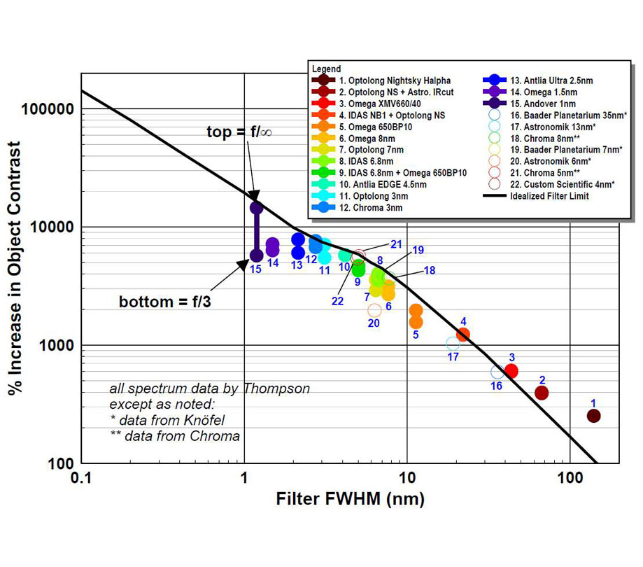
Figure 15 Predicted Contrast Increase: LP w/LED (NELM+2.9), Commercial Filters
The variation in contrast that is delivered by each filter with different f-ratios in general gets larger as the filter FWHM decreases. This relationship is not strongly presented in the available data because other equally important factors are present, such as whether the filter’s CWL is shifted to the left or right of the target wavelength – to the left would increase f-ratio sensitivity, and to the right would decrease sensitivity.
Using the measured filter spectra, I was also able to predict the SNR that would be achieved if each filter was used to collect image data. My calculation assumes a perfect sensor, so both read noise and dark current noise are set to zero. This leaves only shot noise, which scales with the signal, which in turn is the sum of the object luminance and the light pollution luminance. The results of my calculations are presented in Figure 16, again plotted as lines to show how the predicted SNR varies with optics f-ratio. The SNR calculation assumes that sub-exposure time has been kept constant between all the filters being compared. The idealized filter curve corresponding to DC+R=0 has also been included in the plot. As with the contrast plot, almost all the commercially available filters have SNR values at or below the limit line. The impact of f-ratio on SNR is more pronounced than for contrast, i.e., there is a larger difference between SNR values at f/∞ and f/3. The two narrowest filters, #14 and #15 compare very poorly with what is theoretically possible. This observation hints towards a reality regarding how these filters are made; achieving progressively narrower FWHM while maintaining high transmissivity grows progressively more difficult the narrower you go. The difficulty of manufacturing a filter with less than 2nm that is suitable for emission nebula imaging may simply be too prohibitively expensive.
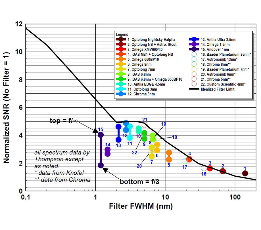
Figure 16 Predicted SNR: LP w/LED (NELM+2.9), Commercial Filters, DC+R=0
The SNR predictions presented in Figure 16 assume that the same sub-exposure time is used regardless of the filter FWHM. In practice, this is not advisable since the signal strength will be proportionally smaller corresponding to the filter’s bandwidth. Because there are physical limits introduced by the sensor, such as bit depth and noise, a more effective approach is to increase the sub-exposure time corresponding to decreasing filter FWHM. Thus, the cost of using a narrower filter, other than its purchase price, is an increase in the length of your sub-exposures. As a rough guide, a filter’s %LT can be used to estimate how much longer a sub-exposure time should be used compared to no filter. For example, a filter with a %LT of 25% would require a sub-exposure time (100/25) 4x what would be used with no filter. Calculated values of %LT for each of the filters considered in this test are provided in Table 2. When these calculated values are plotted versus bandwidth, a simple relationship is evident (see Figure 17). Using this information, the %LT, and thus the recommended sub-exposure time, for any width H-α filter can be estimated.
Figure 17 Calculated %LT vs FWHM for Tested Filters
Astrophotography filters imaging test results
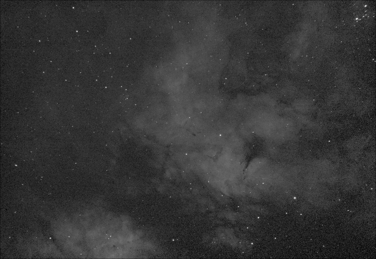
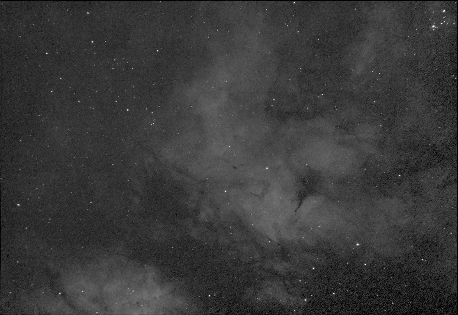
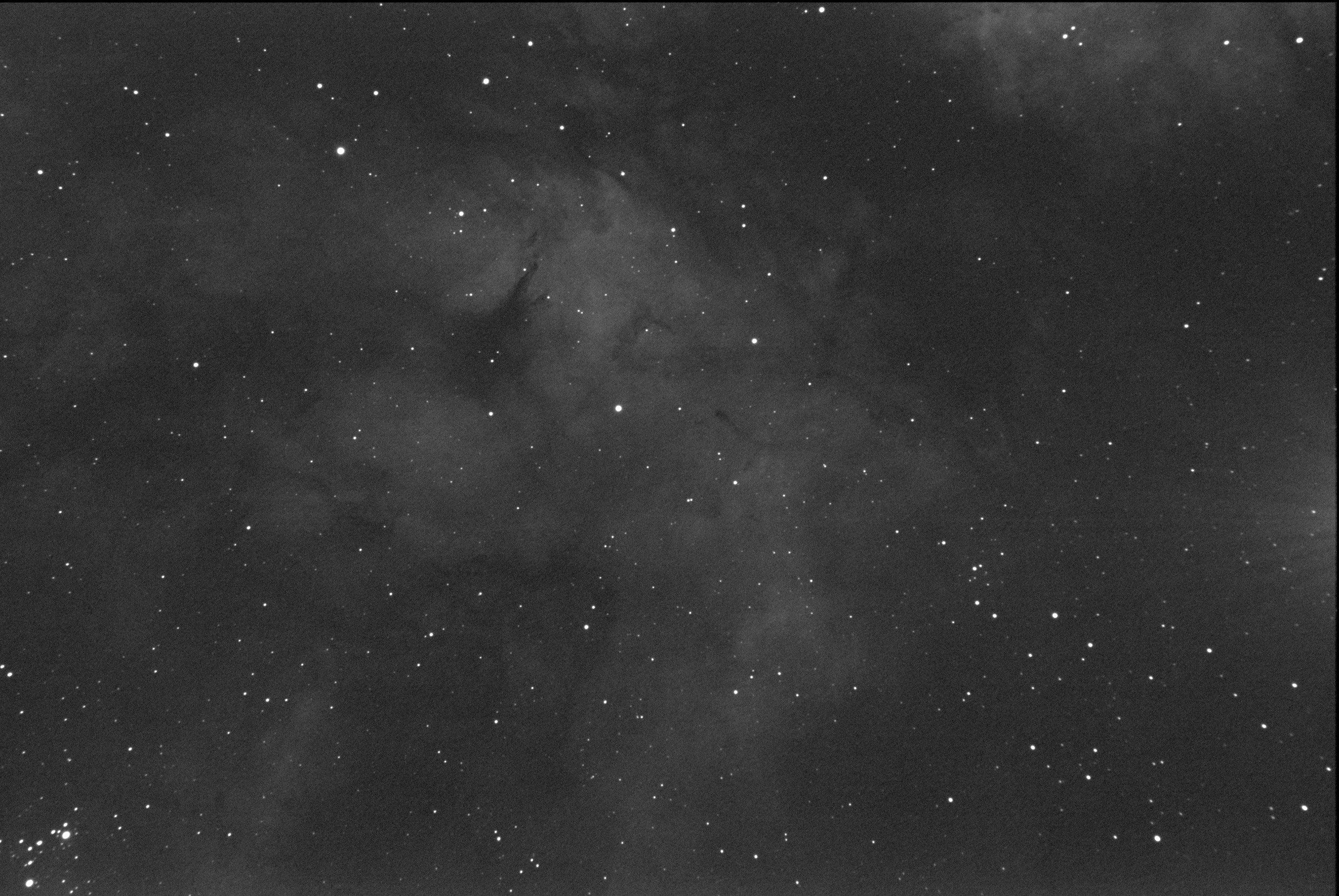
As described above in the Method section, image data was captured during several sessions with each filter using the same scope + camera + target configuration. During each session, all images were collected within a two-hour time window. Data was collected with the ZWO camera by generating a live stack in Sharpcap, which was then saved as a 16-bit FITS file. Images using the Mallincam camera were first captured to disk and then stacked later using Deep Sky Stacker. Two approaches were used regarding sub-exposure time: for some sessions, it was varied according to the %LT of the filter to produce a raw sub-image with roughly the same overall exposure (brightness), and for other sessions, the same sub-exposure time was used for all the filters tested. The number of frames stacked in each case was also varied so that the total exposure time of the final stacked images was the same for each filter in a session.
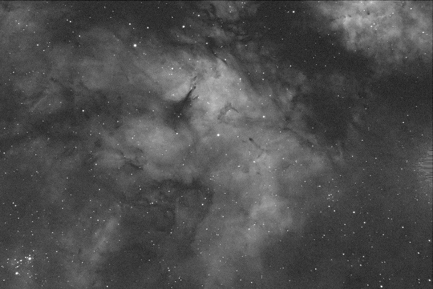
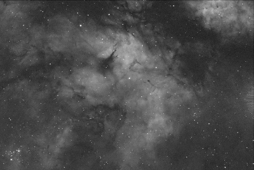
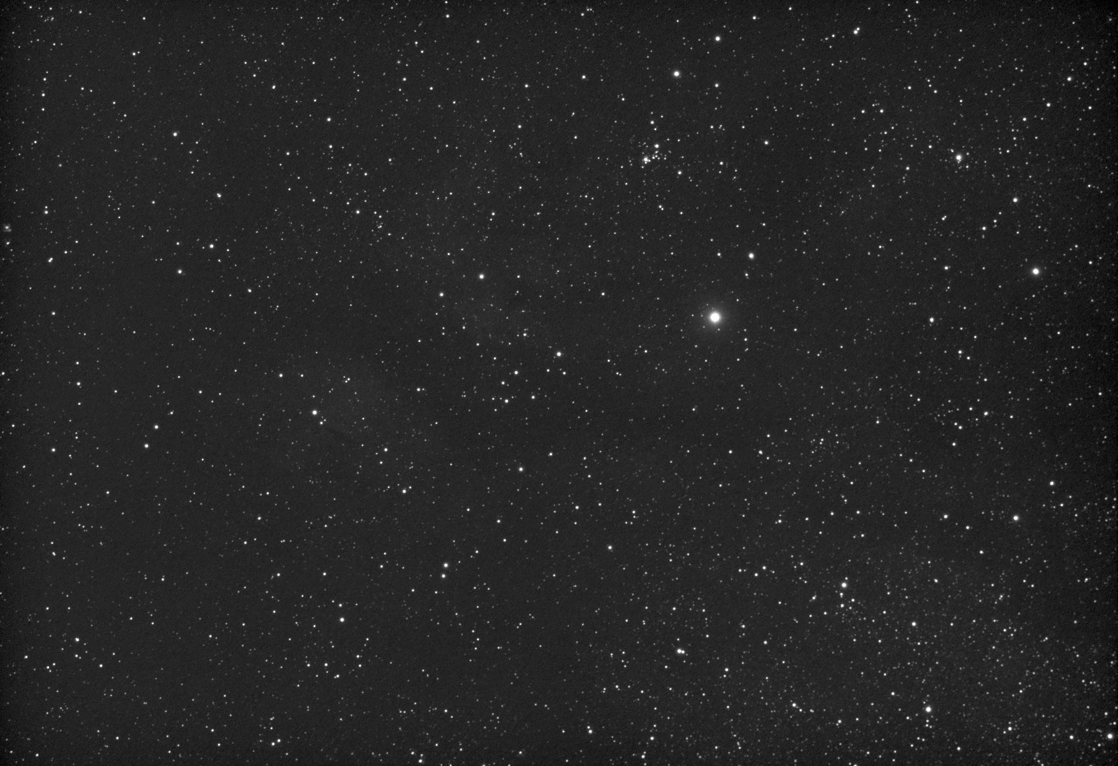
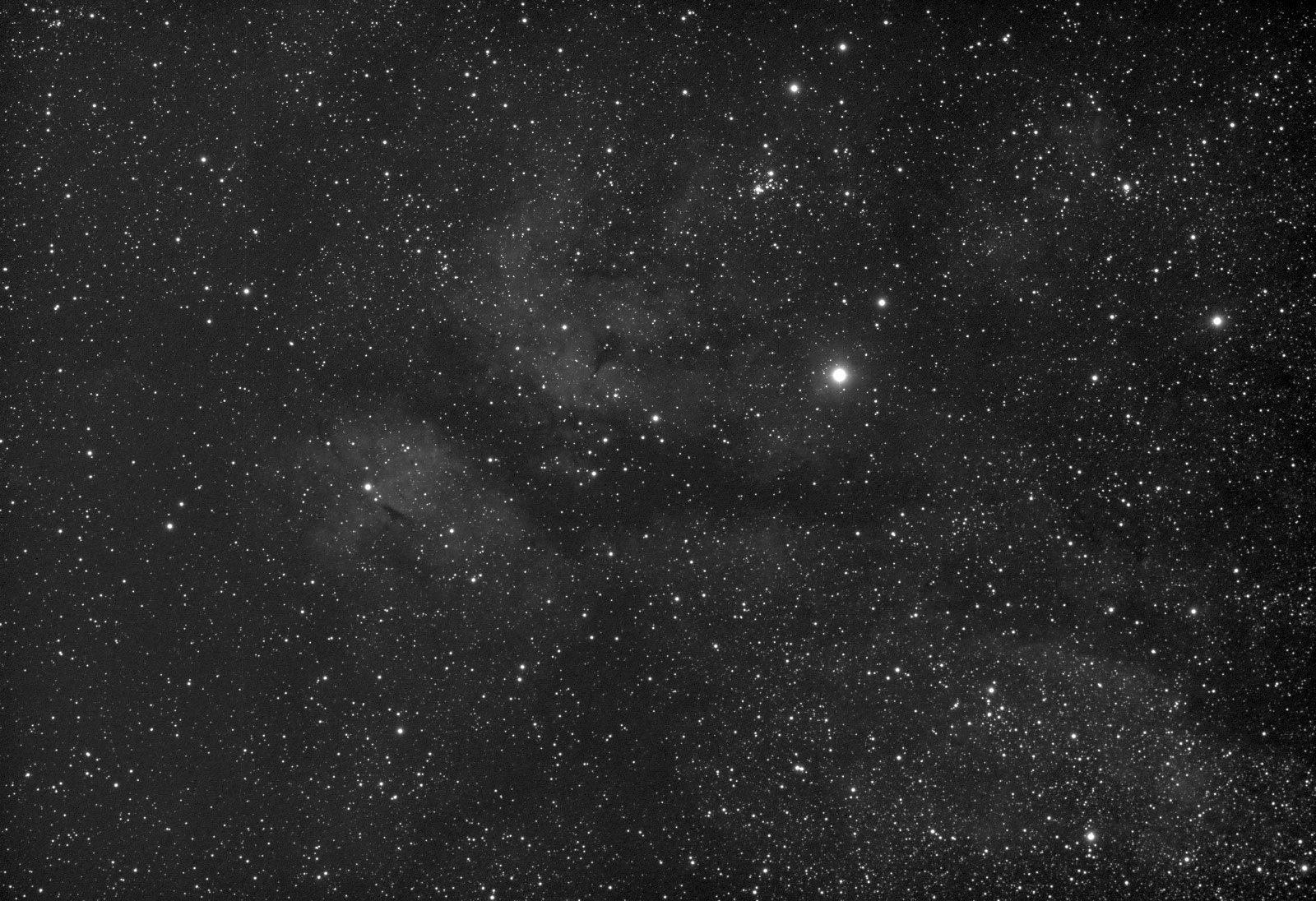
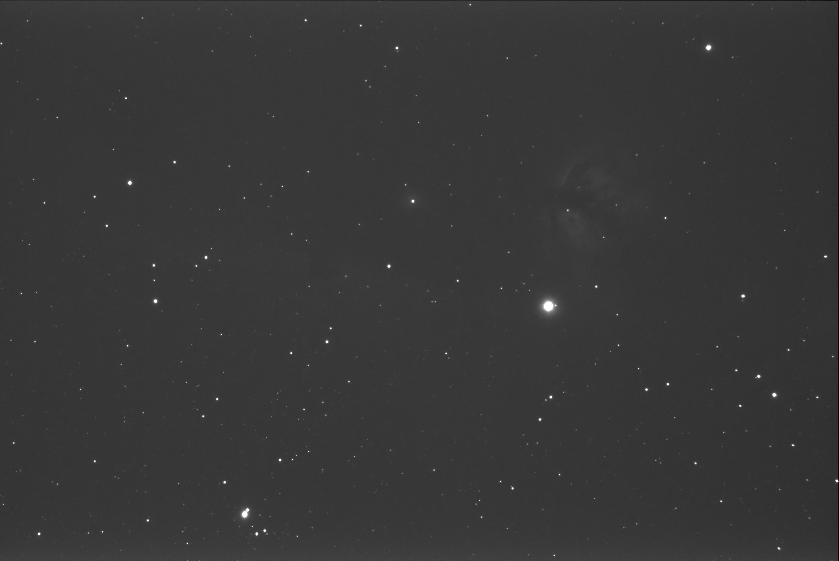
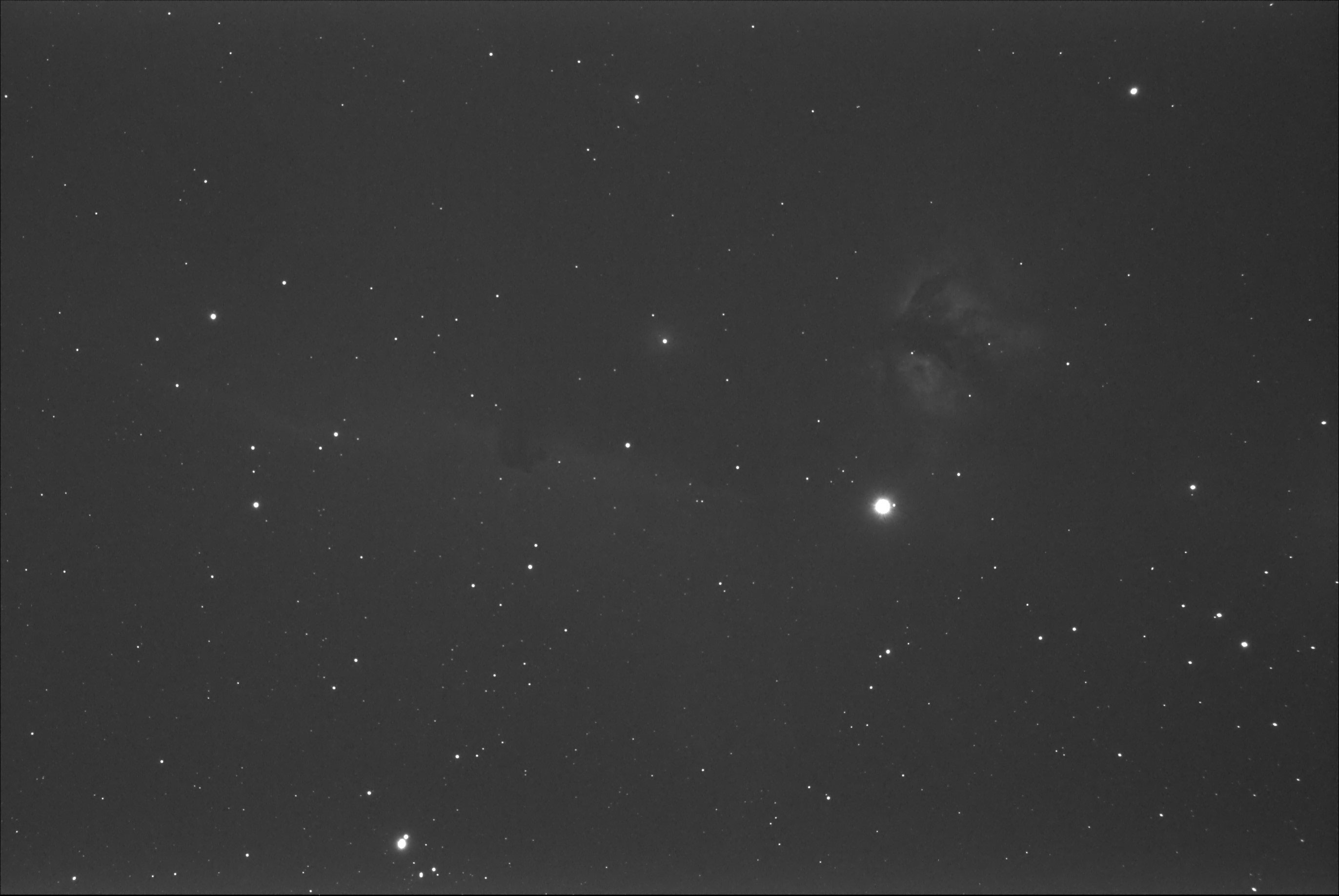
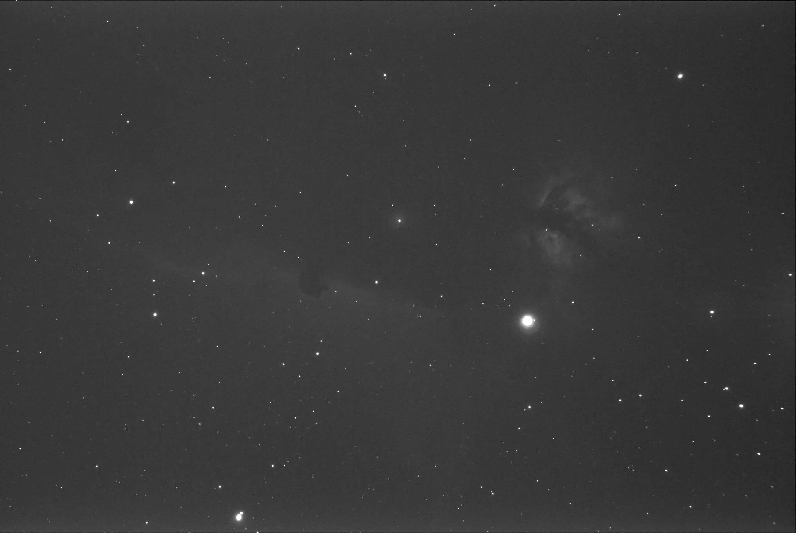
Imaging results from all the sessions can be found in Appendix B. The images presented are of the final stacks and have had their histograms adjusted in the same way using Fitswork v4.47, a free FITS editing software so that they provide as fair a visual comparison as possible. The main thing to note visually from the images is that there is a very obvious change in the extent to which the nebulosity is visible, that extent being more so the narrower the pass band of the filter being used.
Using the captured image data, I was able to directly measure the contrast increase delivered by each filter, putting a number to what was already observed qualitatively from the images. This was accomplished by using AstroImageJ to measure the average luminance from two common areas in the images: a dark background area, and a bright nebulous area. The particular areas used are illustrated in Figure 18, with these same areas used for all the images from the different imaging sessions. The contrast was calculated from the measured luminance values according to Equation 1 presented earlier. Contrast increase was then calculated according to Equation 4.
Equation 4: %Contrast Increase = (Contrastfilter – Contrastno-filter) / Contrastno-filter * 100
, where: Contrastfilter = % contrast measured from image using filter, and Contrastno-filter = % contrast measured from image using no filter.
The resulting contrast increase measurements are plotted in Figure 19 (hollow data markers), and compared with the corresponding predictions for each filter (solid data markers). There was a significant amount of scatter in my measured data, however, there is good alignment between it and my predictions. The large error associated with imaging tests is one of the main reasons I developed the prediction method in the first place. The good agreement between measurement and prediction gives confidence in the prediction method's efficacy.
The measurements of luminance from the images also allowed me to evaluate SNR. When I extracted the average luminance values from each image in AstroImageJ, I also recorded the standard deviation (σ). This allowed me to calculate the SNR achieved by each filter using Equation #3. The measured SNR values are plotted in Figure 20, along with the predicted values for each filter assuming DC+R=0. As with the measured contrast increase values, the measured SNR values show a lot of scatter but align well with predictions. This result provides further evidence that my prediction method can be used for confidently predicting filter performance, including those for which I don’t have a physical sample or hypothetical filters that don’t exist.
An interesting observation coming from my image data is that the Omega 1.5nm filter (#14) tested better than was predicted. The explanation that is immediately evident is that my measurement of that filter’s spectrum may not be accurate; the filter’s peak transmissivity could be higher than I measured. Remeasuring the filter’s spectrum and additional image data would be helpful to confirm if this observation is correct.
Another interesting observation is that since my measurements of SNR align well with predictions for the DC+R=0 case, it implies that the actual dark current signal noise plus read noise magnitudes for my particular cameras are very low; near zero relative to the shot noise.
Cost-effectiveness
In addition to answering the primary question about the practical limits on bandwidth, I also set out in this test to evaluate filter cost-effectiveness. Using my predictions of SNR, now validated against measured data, I have assembled a plot of $USD per unit SNR versus FWHM (see Figure 21). There was a lot of scatter found for the list of filters considered in my test, their cost-effectiveness varying widely from $50 per unit SNR to over $300. In general, the spread and peak cost of the filters increases with decreasing bandwidth. The data implies, however, that there are three classes of filter: bargain (<$100/SNR), good value ($100/SNR to $150/SNR), and premium (>$150/SNR). To further refine and populate these three classes I decided to survey all the H-α filters available today for commercial sale. A list of the resulting 41 filters is provided in Table 3. For all of these filters, I predicted a normalized SNR value, either using the measured spectra as was the case for all the filters considered in my testing or by simply using the peak %LT and FWHM values quoted by the filter manufacturers. A summary of my filter survey data is available in Appendix C, sorted by increasing FWHM. This allowed me to plot a master cost-benefit graph; price versus SNR for each filter. The resulting graph is presented in Figure 22. The numbers inside each data marker correspond to the filter numbers listed in Table 3. The data marker color corresponds to the calculated $USD per unit SNR. Figure 22 makes it clear that regardless of the performance level (i.e., SNR) you wish to achieve, there is a filter available for sale in every price class: bargain (purple/dark blue markers), good value (blue/green markers), or premium (yellowish-green/yellow/orange/pink markers). In the last couple of years, there has
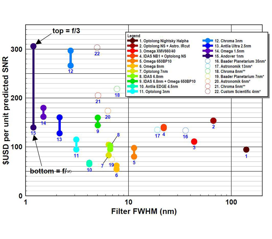
Figure 21 Filter $USD per Unit Predicted SNR
Table 3 List of Commercially Available H-α Filters
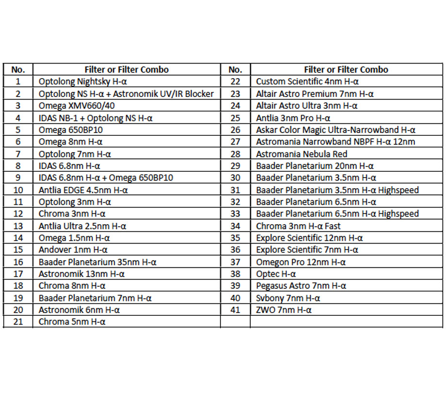
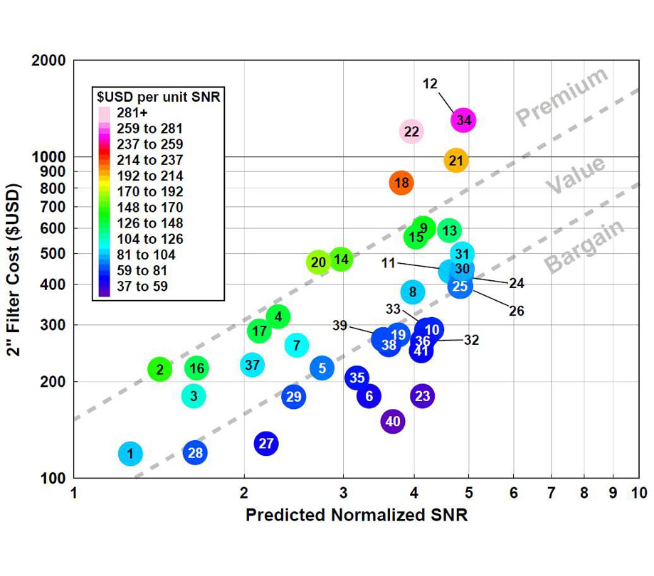
Figure 22 Filter $USD per Unit Predicted SNR
been a lot of growth in the number of different filter models and brands available in this class, most notably from Chinese manufacturers. These new brands are providing serious competition against the “premium” brands, offering “good value” and “bargain” priced products with premium features like very narrow FWHM, high off-band blocking (>OD4) to eliminate halos, and per-batch measured filter spectra. If someday filters were to be available narrower than 2.5nm, the narrowest currently available for amateur astronomy use, Figure 22 gives an idea of what they might cost. For example, a 2” diameter 1nm filter (SNR ~6.5) from a “premium” supplier should be in the $1000-$2000USD range. From a “good value” supplier the same filter should be in the $500-$1000USD range, and though unlikely, $250-$500USD from a “bargain” supplier. Manufacturing such narrow filters with any amount of repeatability will be expensive and require serious quality control, which in my opinion puts them into the premium filter price category by default.
Conclusions
Based on the results of the analysis and testing described above, I have made the following conclusions:
-
Contrast: For the range of FWHM considered, there was no limit observed in nebula contrast increase that could be realized using a progressively narrower bandwidth. Contrast increases monotonically as FWHM decreases. This conclusion is based primarily on analysis, but imaging results were found to be consistent with predictions. The two sub-2nm sample filters available for testing were found to be poor representations of what should be possible with a filter purpose-built for astronomy. Also of note is that there is a small discontinuity in the predicted contrast versus FWHM that is a result of secondary nebula emissions with wavelengths adjacent to the emissions of interest.
-
SNR: For the range of FWHM considered, there was no limit observed in nebula SNR that could be realized using a progressively narrower bandwidth. The magnitude of the benefit, however, is dependent on the LP level and the camera noise (dark current signal noise + read noise). Less LP and/or more camera noise reduces the effectiveness of a progressively smaller FWHM. This conclusion is based primarily on analysis, but imaging results were found to be consistent with predictions. The two sub-2nm sample filters available for testing were found to be poor representations of what should be possible with a filter purpose-built for astronomy. Also of note is that there is a moderate amplitude discontinuity in the predicted SNR versus FWHM that is a result of secondary nebula emissions with wavelengths adjacent to the emissions of interest. The discontinuity results in a range of FWHM values for which there are only small differences in SNR predicted. For H-α filters this range is from 2 to 5nm, for O-III 7 to 12nm, and for S-II 1 to 10nm.
-
F-ratio Sensitivity: Due to how narrowband filters function, through a combination of constructive and destructive light interference, they are sensitive to the angle at which light passes through the filter and thus sensitive to telescope f-ratio. This sensitivity is larger for smaller FWHM, limiting the usability of very narrow filters to slower f-ratios. FWHM values below 2nm are probably not practical for the general amateur astronomer market for this reason.
-
Sub-Exposure Time: As FWHM decreases, so does the amount of light passing through the filter. Maintaining the optimum usage of the camera dynamic range requires sub-exposure time to be increased in conjunction with decreasing FWHM. Filter %LT can be used to estimate how much longer one’s sub-exposures need to be compared with no filter. For a 10nm H-α filter, a sub-exposure of approximately 50x that of no filter is required, and for a 1nm filter about 500x.
-
Cost: To be able to fabricate filters with FWHM values below 2nm that are useful for amateur astronomy would be difficult and expensive. Such filters would require %LT values above 80% (preferably >90%), off-band blocking better than OD4, and CWL accuracy better than ±0.2nm. Based on the price-per-performance of existing commercially available filters, the price expected for a 2” diameter 1nm wide filter would be between $1000 and $2000 USD.
-
Bottom Line: Although there would seem to be no limit on the imaging performance improvements that can be realized with progressively narrower filters (down to 0.1nm wide at least), that does not mean that there isn’t a practical limit on what is useful to amateur astronomers. The increase in performance that you get from narrower FWHMs comes at a cost of longer sub-exposure times, higher sensitivity to optics f-ratio, and higher purchase prices. For astrophotographers who image at different f-ratios, it would be very inconvenient if they needed a different filter, optimized for band shift, for each of their telescope setups. With all things considered, there would appear to be no practical reason to go below a FWHM of 2nm. For H-α filters, there is only a small SNR difference predicted for filters in the 2 to 5nm range, so any filter in that range can be considered near-optimum.
Appendix A – Idealized filter performance predictions
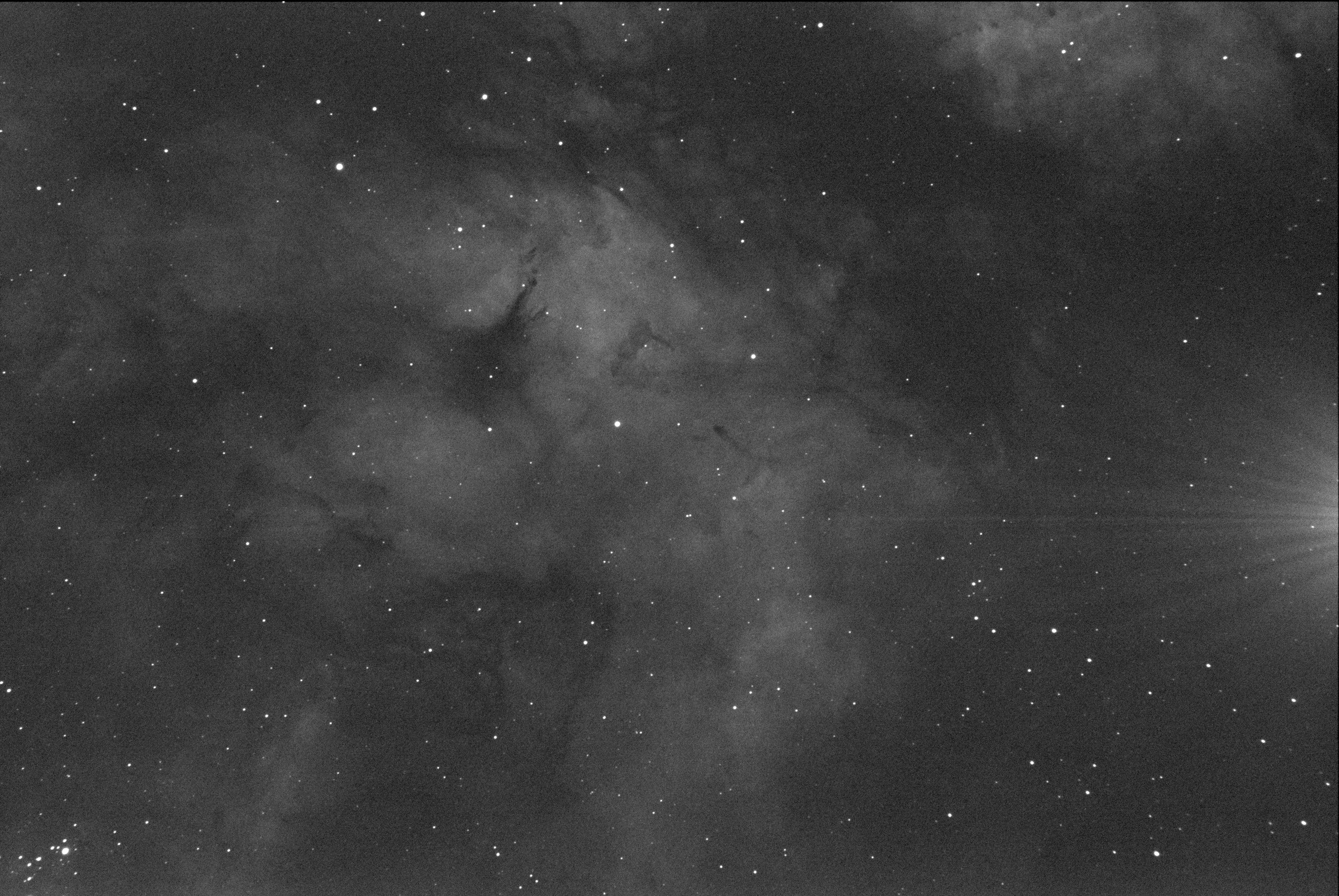
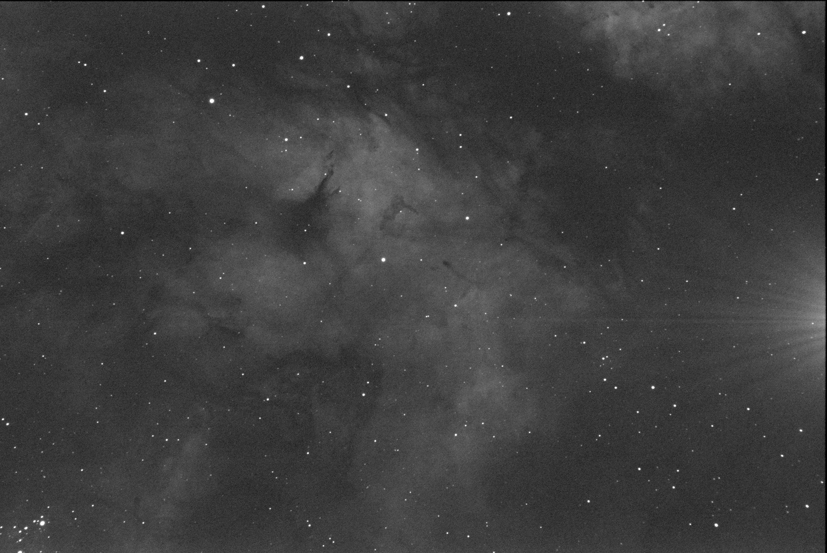
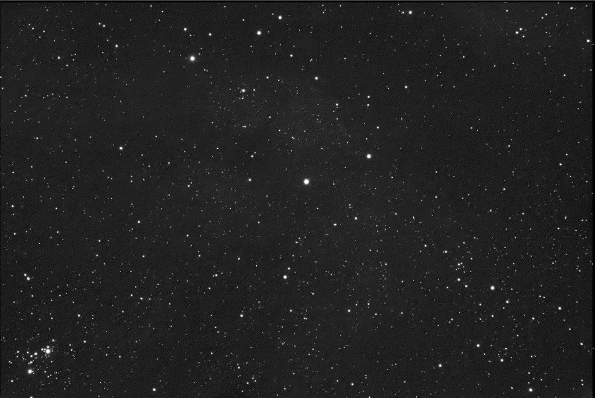
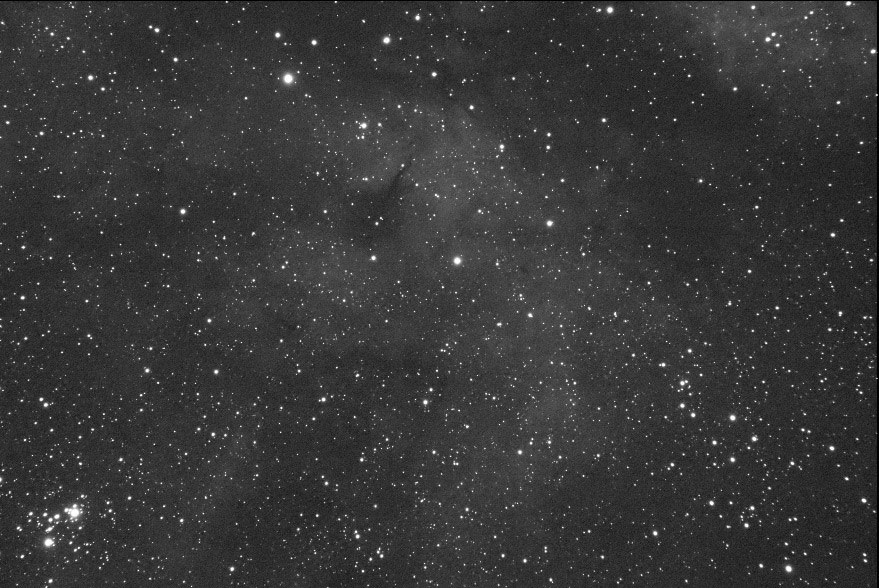
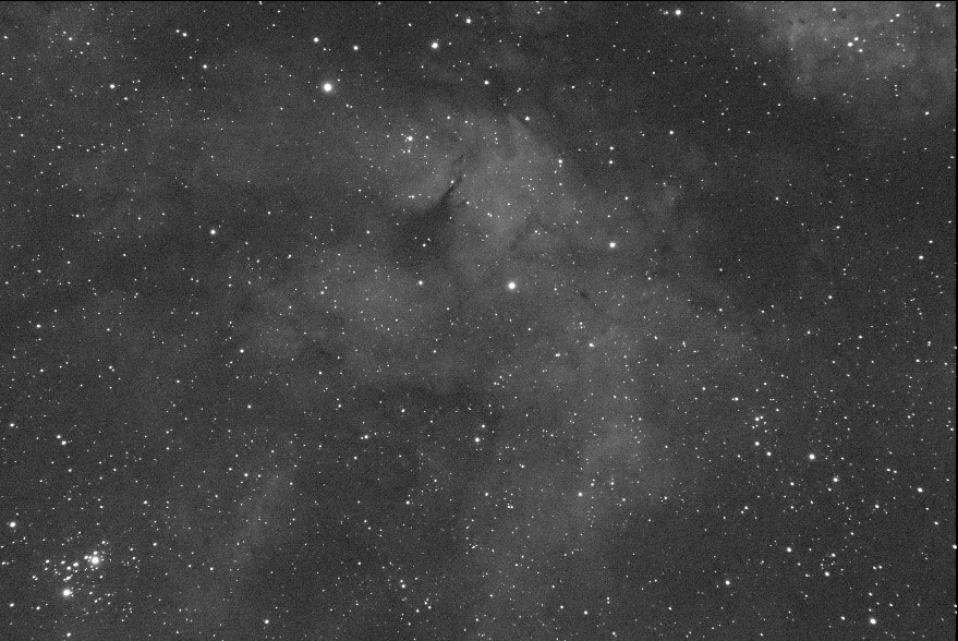
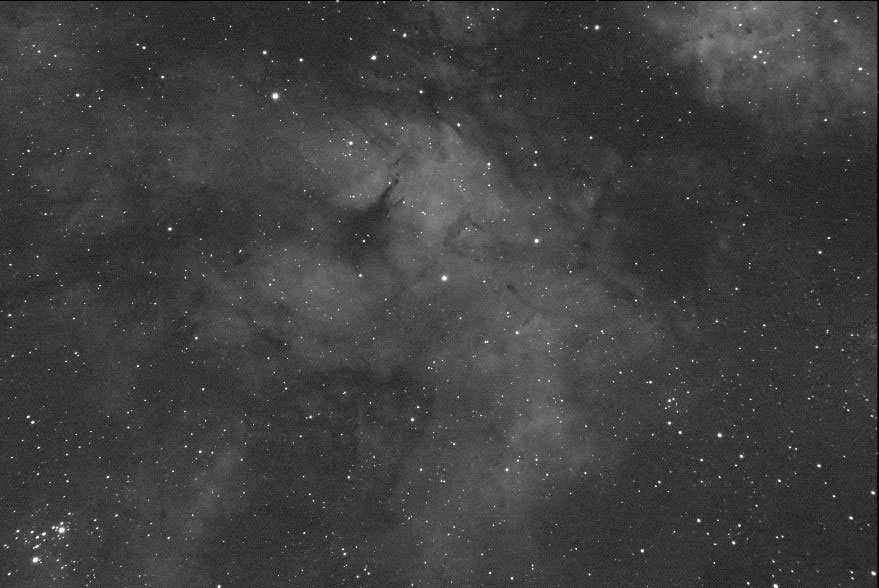
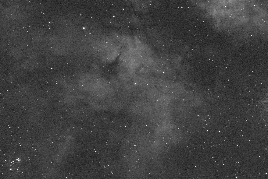
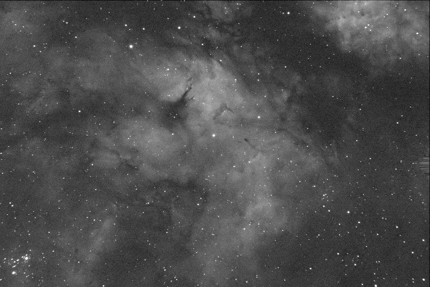
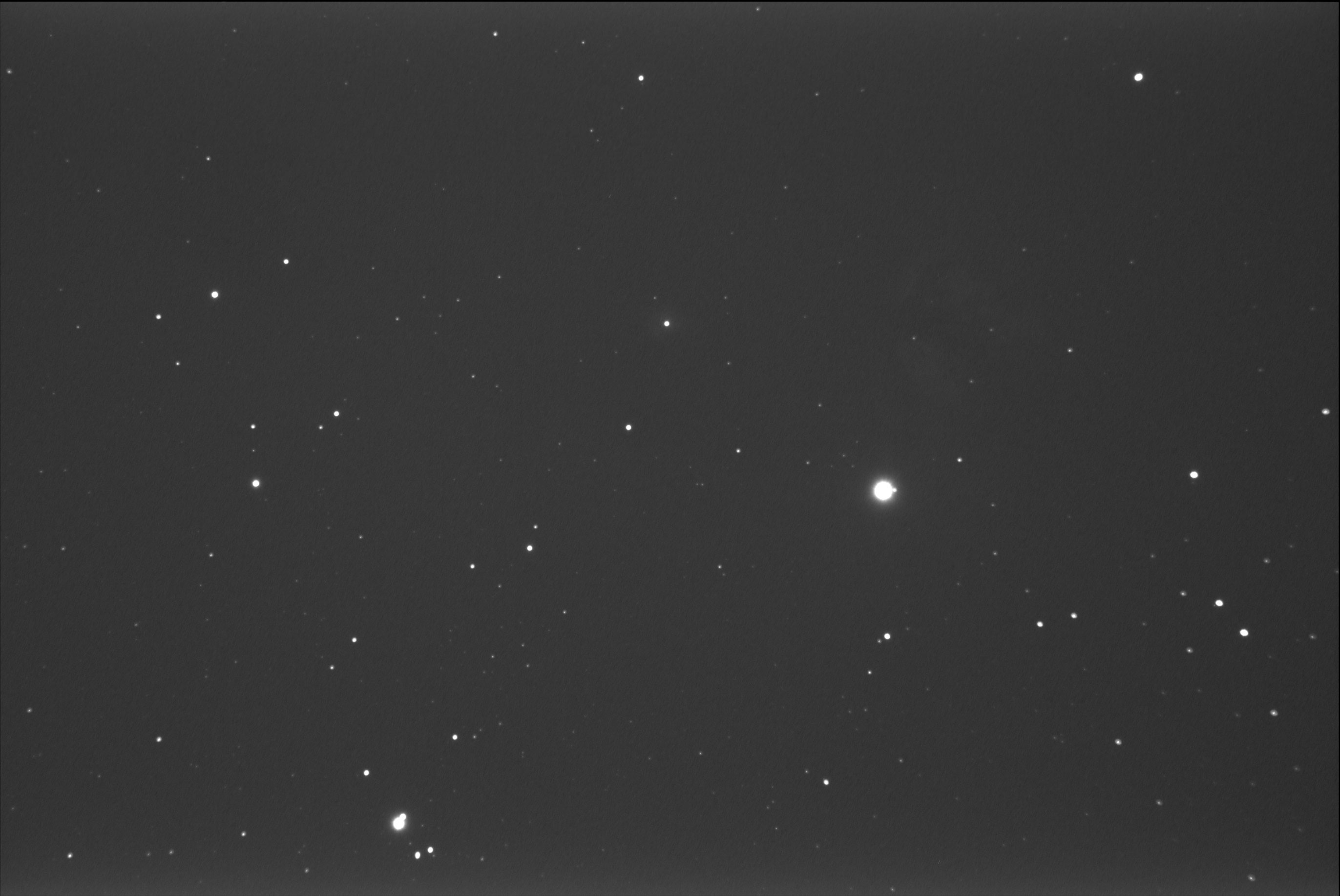
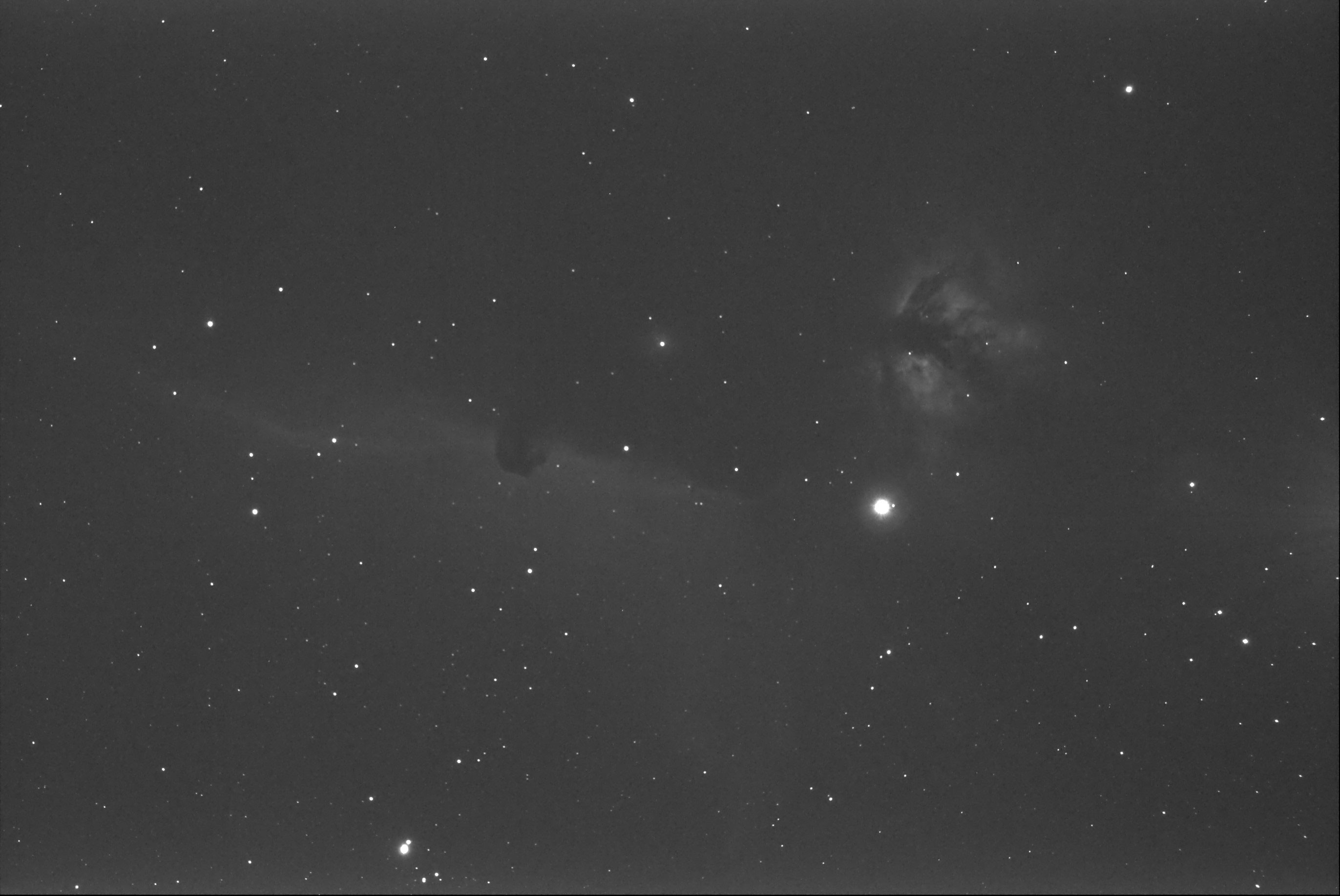
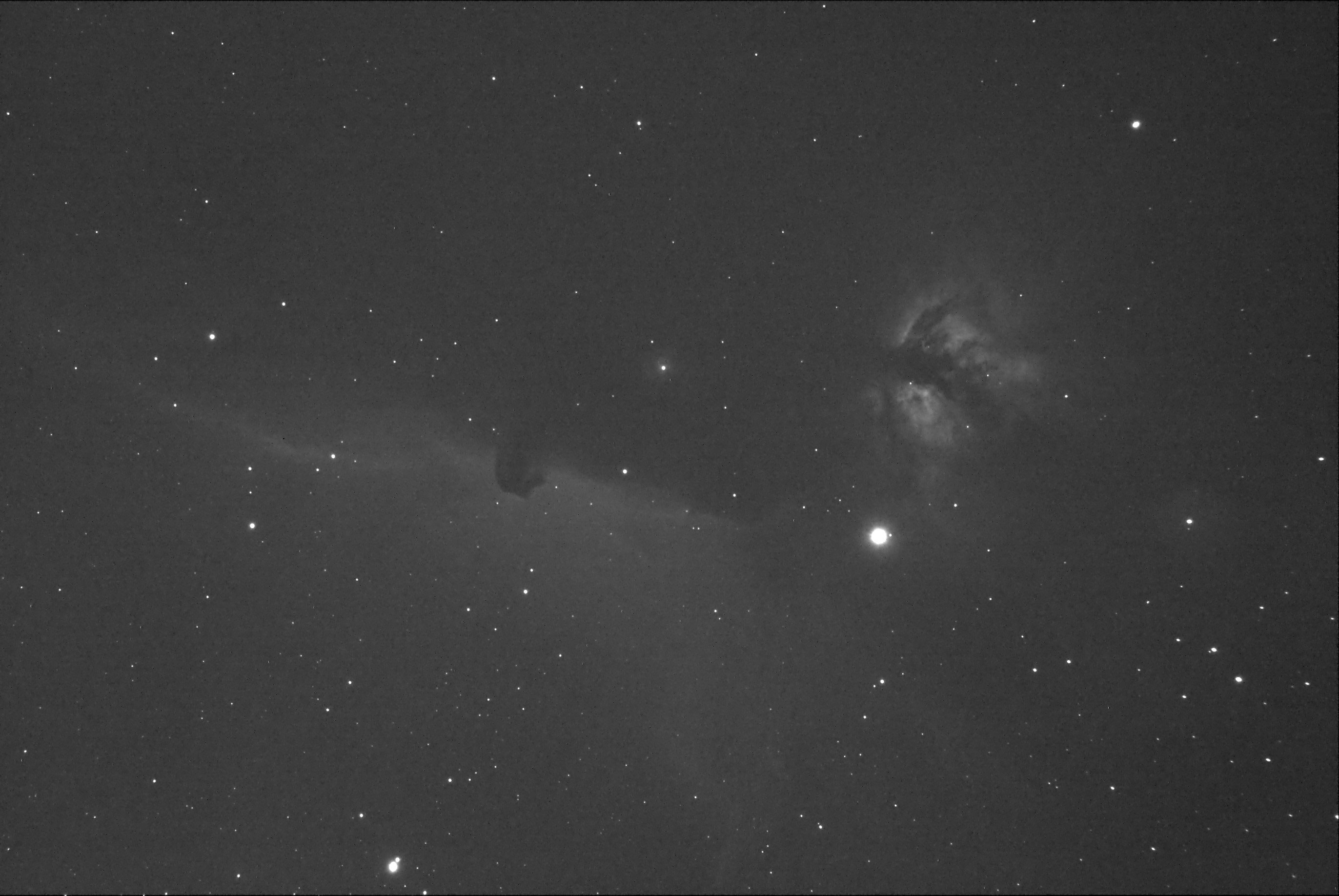
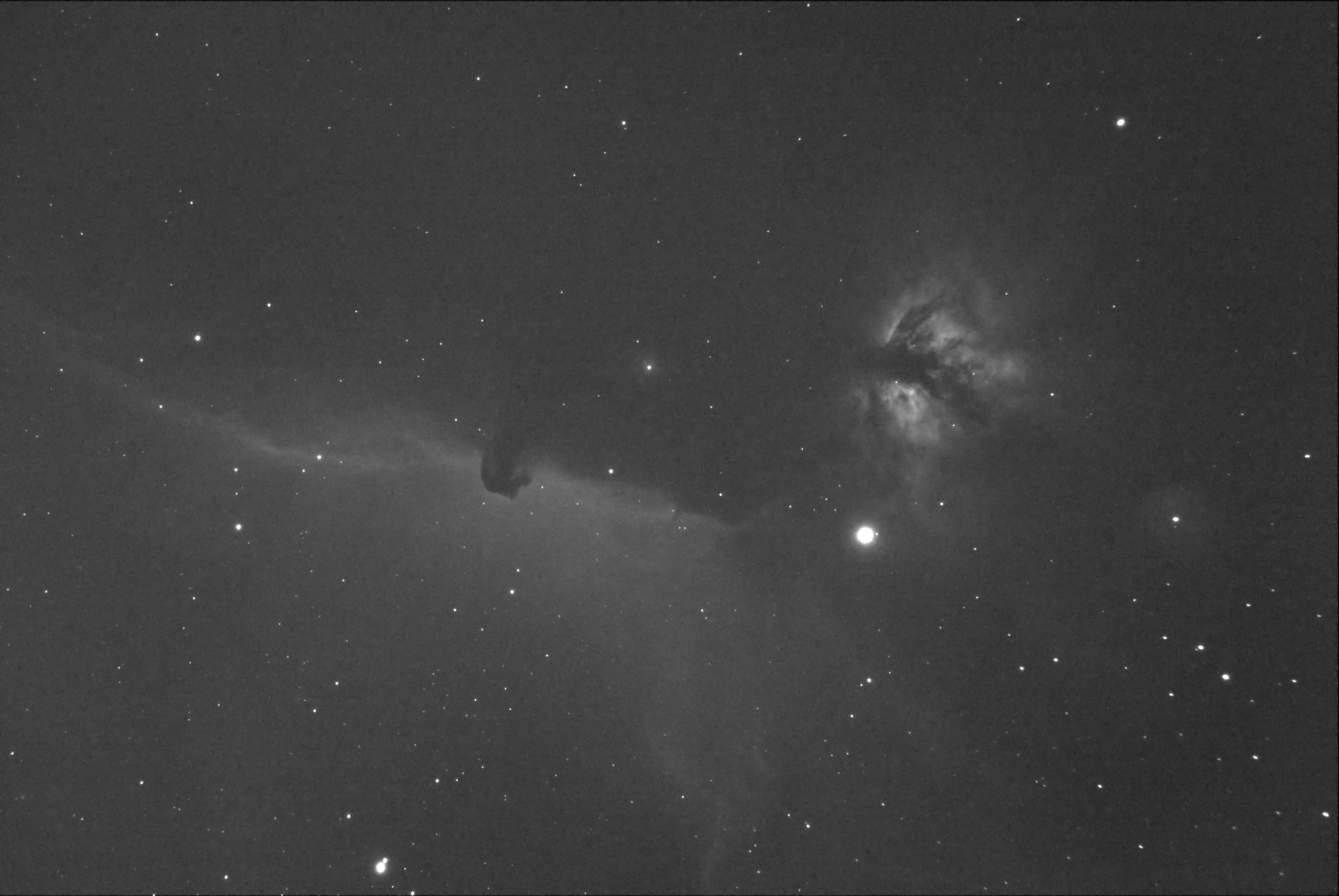
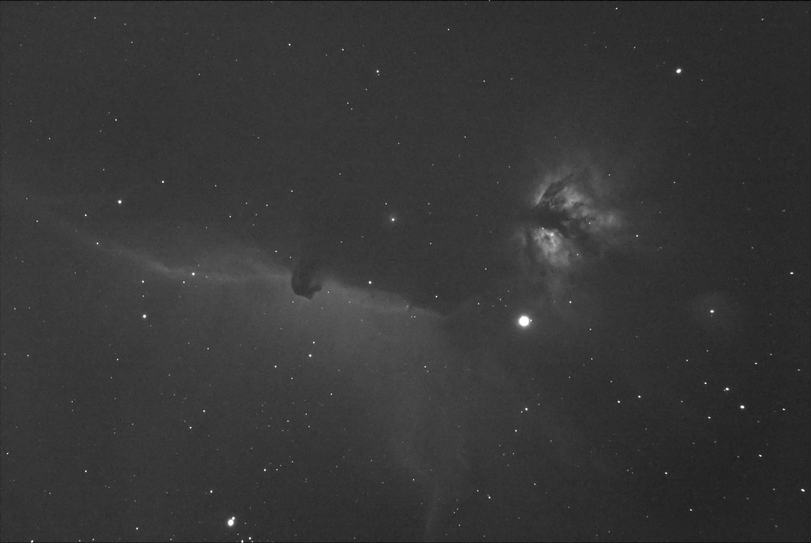
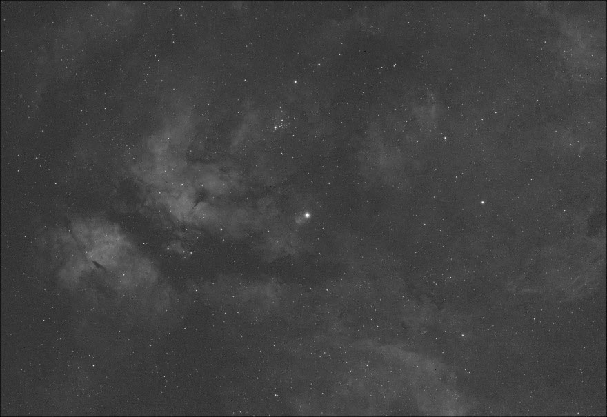
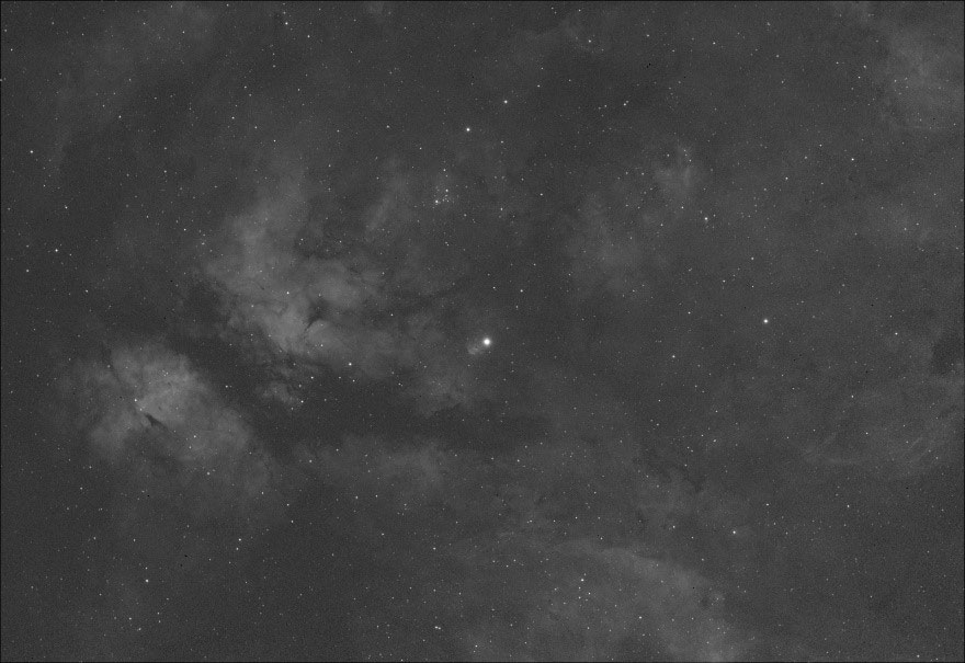
Session #1 - June 12th, 2022 imaging results
0. No Filter (91 x 4s)
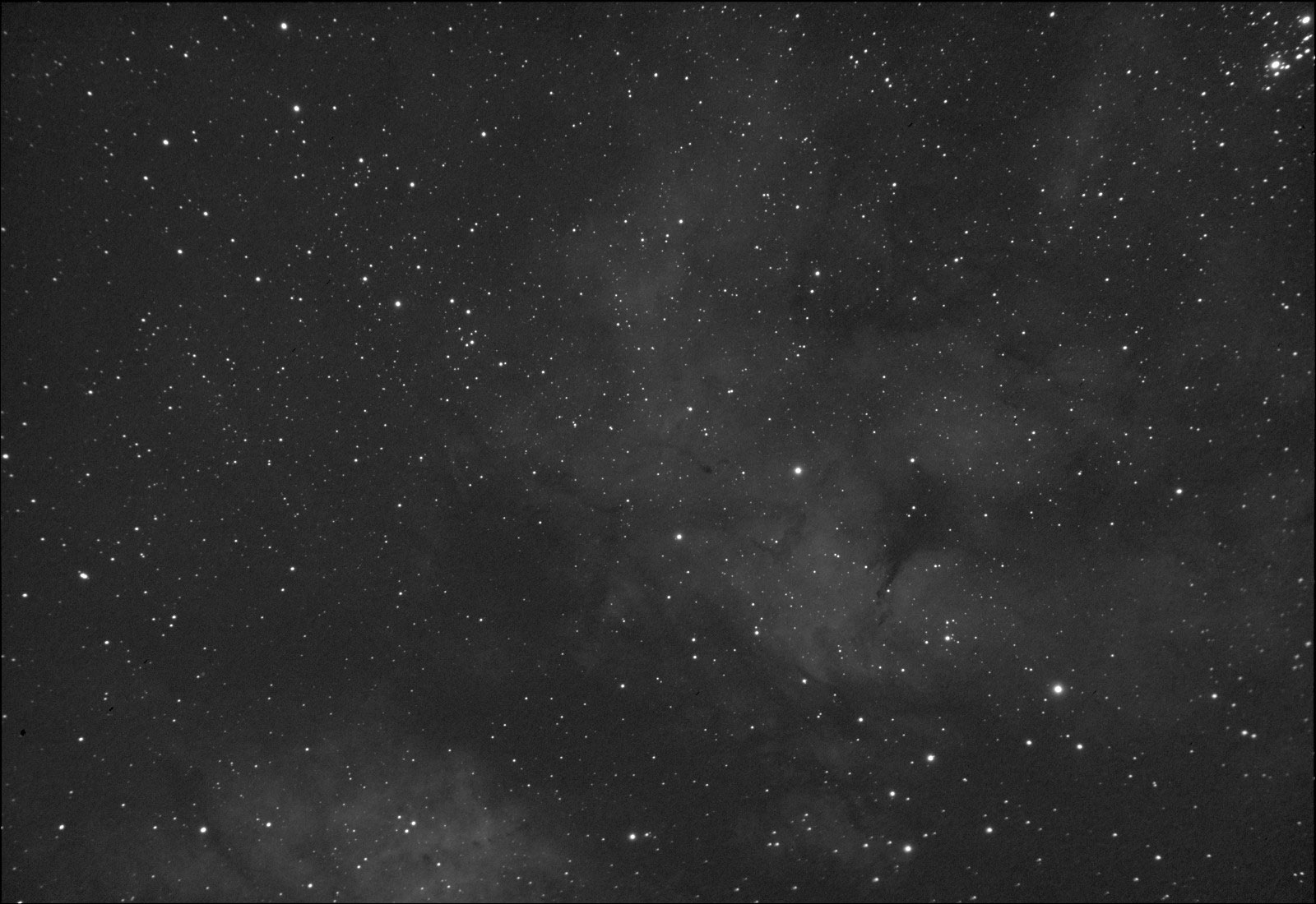
3. Omega XMV660/40 (30 x 20s)
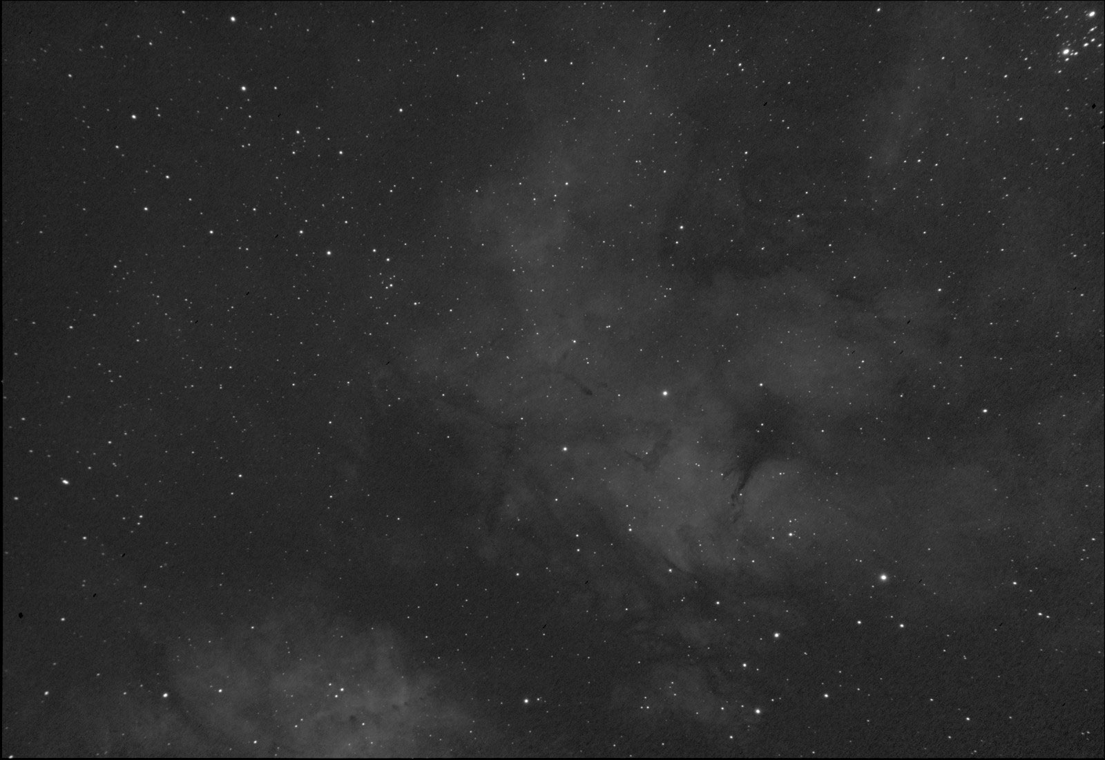
5. Omega 650BP10 (30 x 20s)
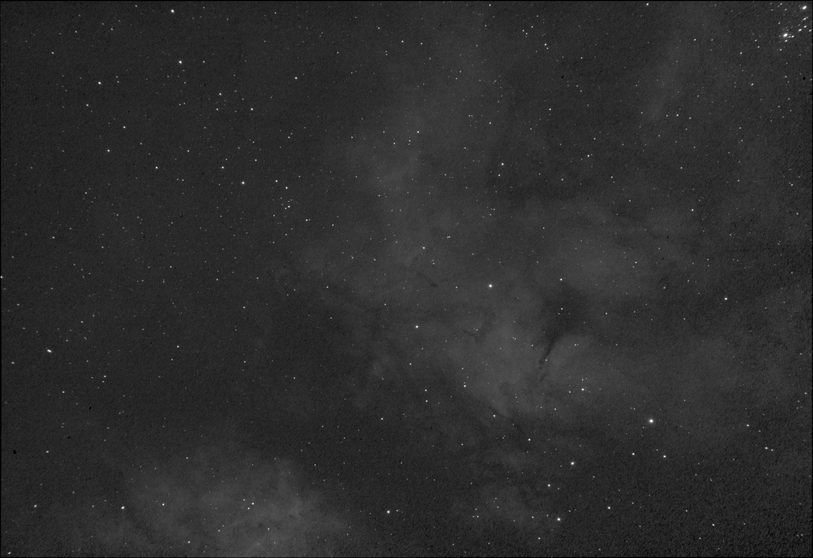
7. Optolong 7nm (30 x 20s)
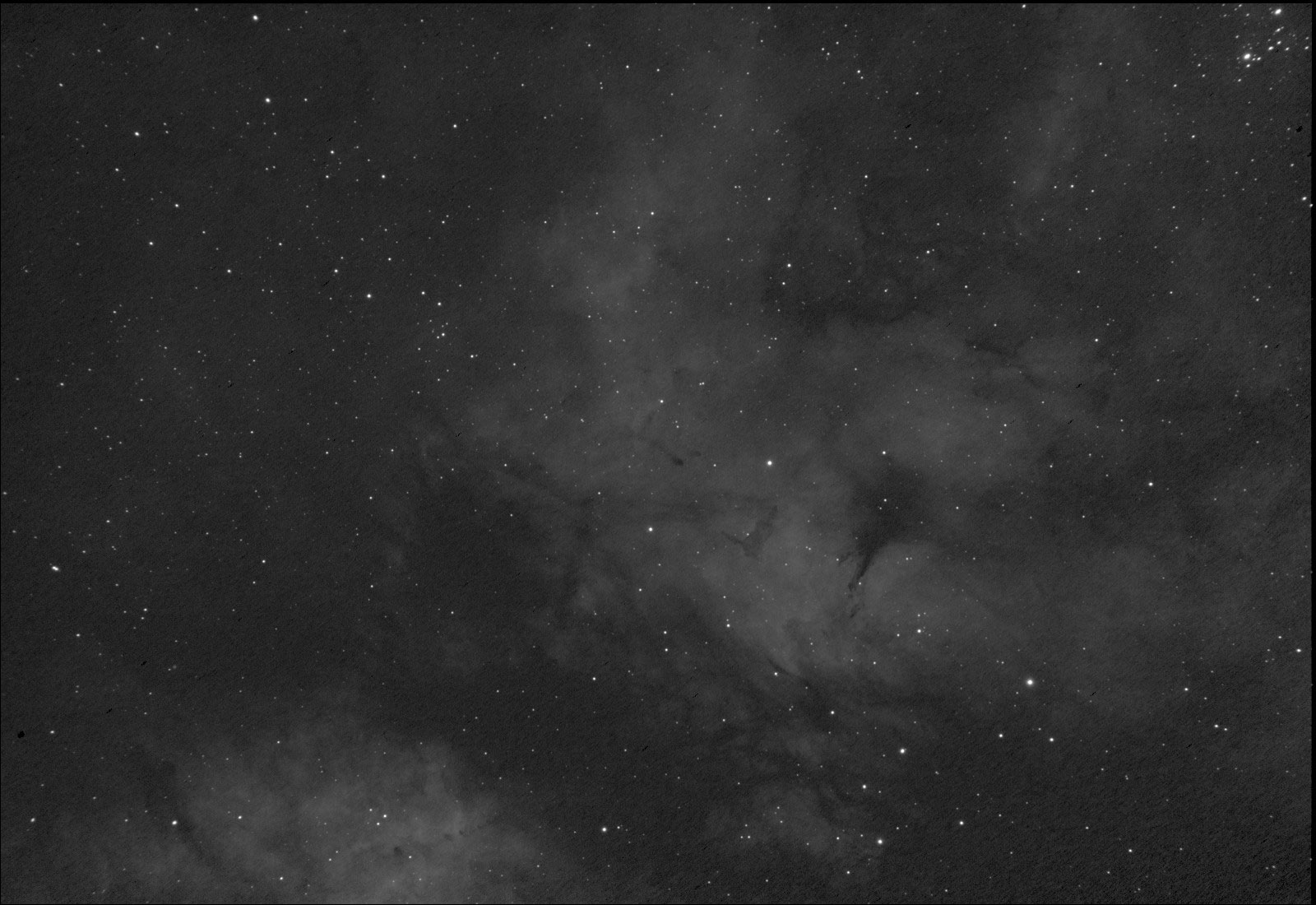
8. IDAS 6.8nm (30 x 20s)
11. Optolong 3nm (30 x 20s)
12. Chroma 3nm (30 x 20s)
Session #2 - June 16th, 2022 imaging results
0. No Filter (180 x 2s)
8. IDAS 6.8nm (12 x 30s)
11. Optolong 3nm (6 x 60s)
12. Chroma 3nm (6 x 60s)
Session #3 - June 24th, 2022 imaging results
0. No Filter (300 x 1s)
1. Optolong Nightsky H-α (40 x 7.5s)
3. Omega XMV660/40 (15 x 20s)
5. Omega 650BP10 (8 x 40s)
7. Optolong 7nm (4 x 75s)
8. IDAS 6.8nm (4 x 75s)
11. Optolong 3nm (3 x 120s)
12. Chroma 3nm (3 x 120s)
Session #4 - June 28th, 2022 imaging results
0. No Filter (600 x 1s)
1. Optolong Nightsky H-α (60 x 10s)
3. Omega XMV660/40 (20 x 30s)
5. Omega 650BP10 (8 x 75s)
8. IDAS 6.8nm (5 x 120s)
11. Optolong 3nm (4 x 180s)
Session #5 - February 6th, 2023 imaging results
0. No Filter (700 x 0.5s)
1. Optolong Nightsky H-α (265 x 1.3s)
2. Opto. NS H-α + Astro. IR Cut (91 x 3.9s)
3. Omega XMV660/40 (58 x 6.1s)
4. IDAS NB-1 + Opto. NS H-α (35 x 10s)
5. Omega 650BP10 (18 x 19s)
8. IDAS 6.8nm (10 x 35s)
9. IDAS 6.8nm + Omega 650BP10 (8 x 44s)
11. Optolong 3nm (5 x 70s)
14. Omega 1.5nm (2 x 175s)
15. Andover 1nm (1 x 350s)
Session #6 - February 8th, 2023 imaging results
8. IDAS 6.8nm (5 x 120s)
11. Optolong 3nm (5 x 120s)
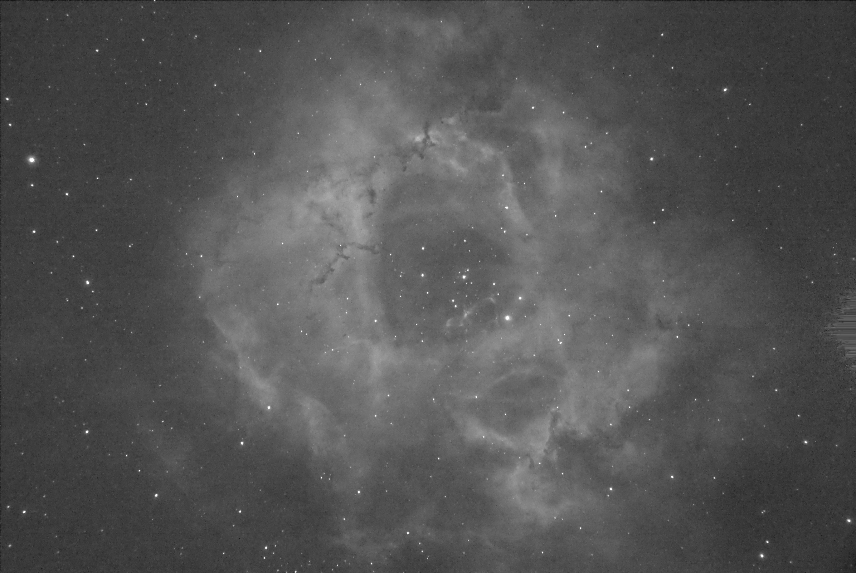
14. Omega 1.5nm (5 x 120s)
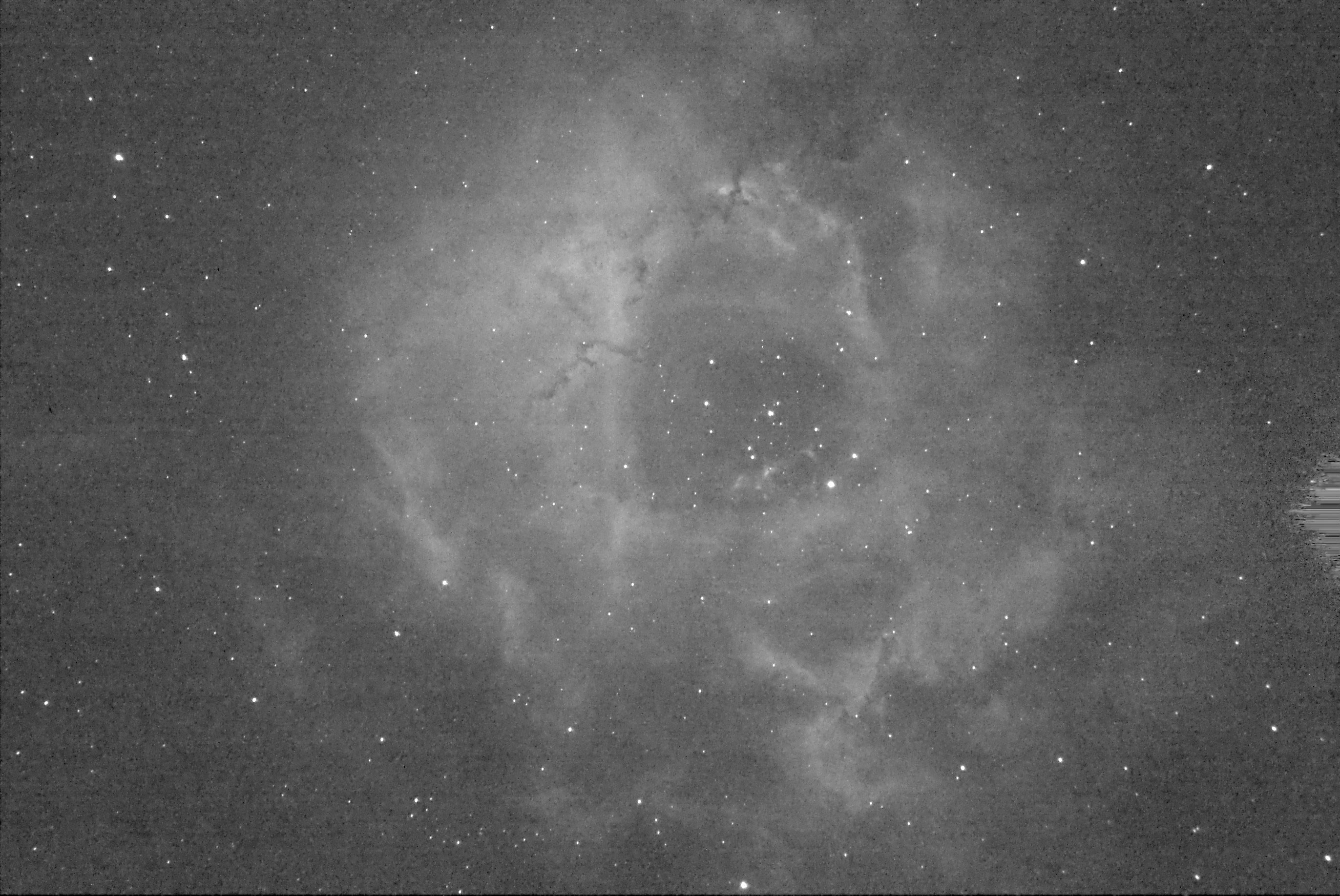
15. Andover 1nm (5 x 120s)
Session #7 – July 27th, 2023 imaging results
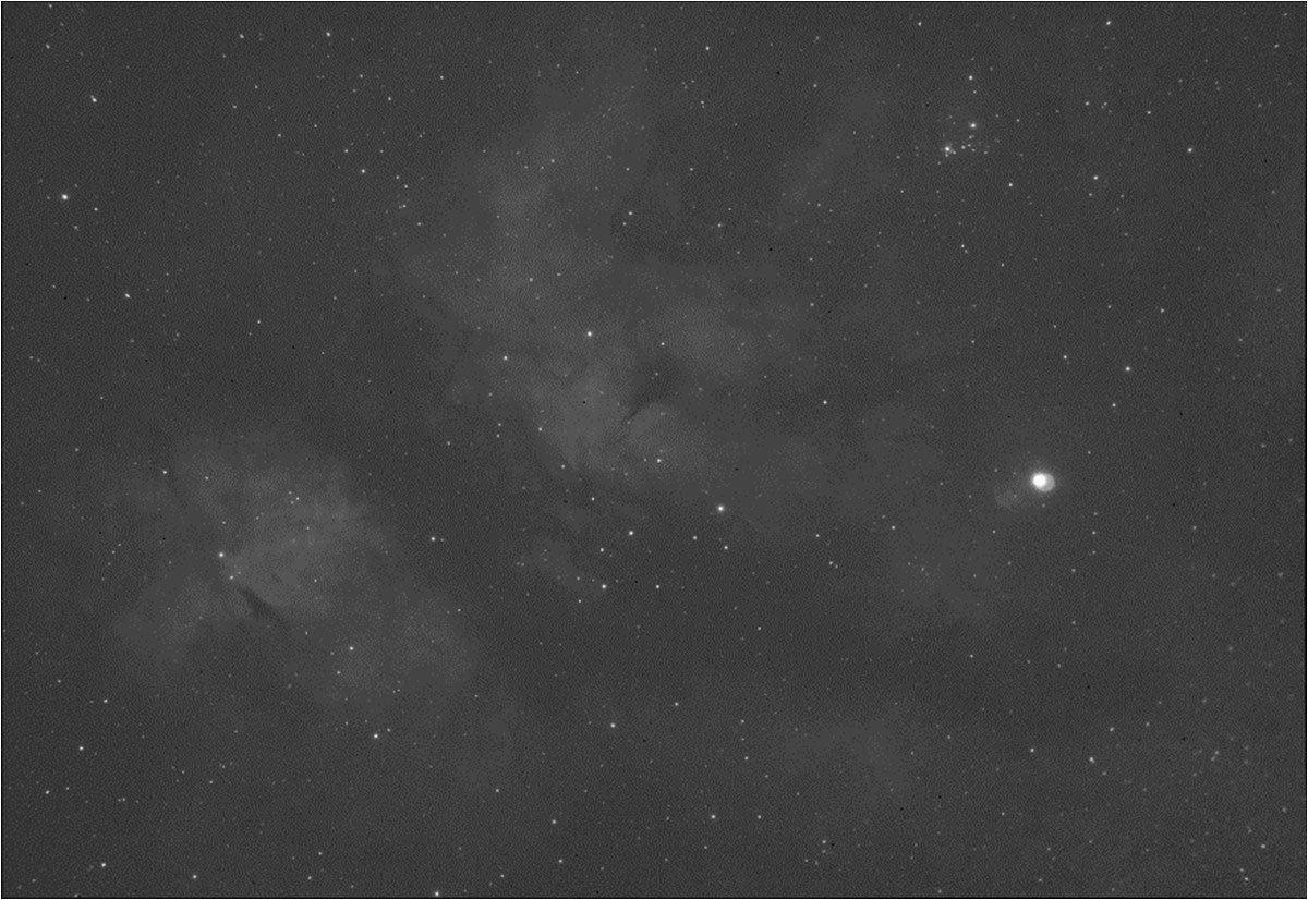
6. Omega 8nm (20 x 30s)
8. IDAS 6.8nm (20 x 30s)
10. Antlia Edge 4.5nm (20 x 30s)
11. Optolong 3nm (20 x 30s)
13. Antlia Ultra 2.5nm (20 x 30s)
14. Omega 1.5nm (20 x 30s)
Session #8 – August 1st, 2023 imaging results
8. IDAS 6.8nm (30 x 20s)
10. Antlia Edge 4.5nm (18 x 34s)
11. Optolong 3nm (14 x 44s)

13. Antlia Ultra 2.5nm (12 x 54s)
Appendix C – H-alpha Filter Cost vs. Performance Summary Table
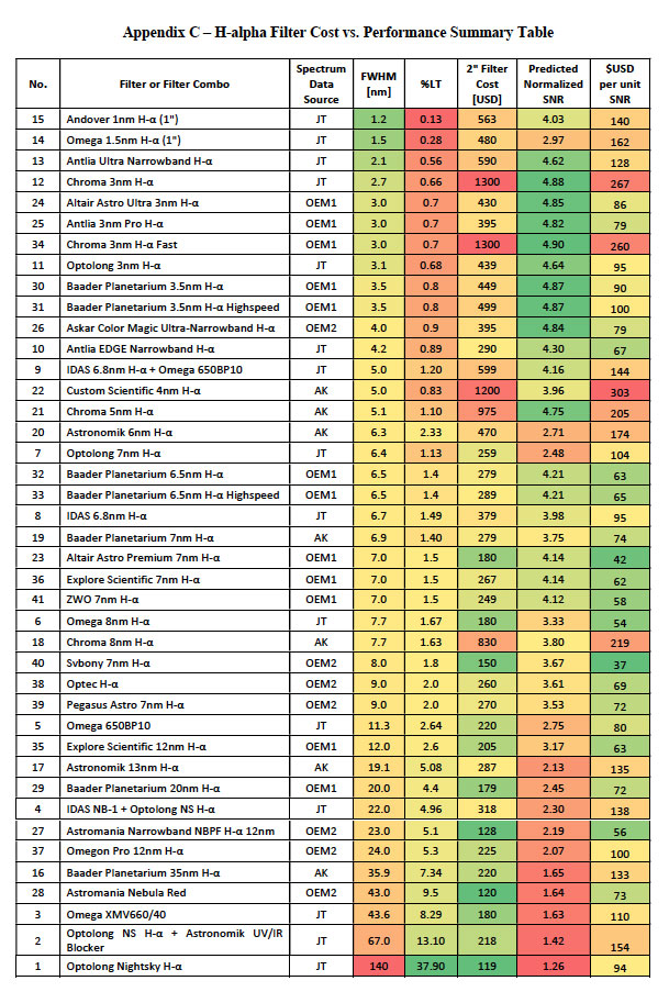
Spectrum data sources
JT measured by Jim Thompson
AK measured by André Knöfel
C measured by Chroma Filters
OEM1 values of FWHM & peak %LT quoted by filter manufacturer were used as-is
OEM2 values of FWHM & peak %LT extracted from spectrum plot issued by manufacturer
ScopeTrader's latest survey
Featured Stories


Stay Updated
Sign up for our newsletter for the headlines delivered to youSuccessFull SignUp

|

Comments